Automate Model Preprocessing with the Application Builder

Have you ever wanted to rapidly set up a COMSOL Multiphysics model with hundreds of different parts? If so, you might not want to use a graphical user interface where you manually enter dimensions and properties for each part. Generating a text file that contains all of this information offers a much faster route. Today, we will look at how you can use the Application Builder to quickly convert a text input file into a COMSOL model.

Quickly and Easily Define Your Models with the Application Builder

Suppose that you have been tasked with performing thermal analyses on many different circuit boards, such as the one pictured below. Notice that there are a lot of different chips, resistors, capacitors, and other components on the board. The data that you have been given includes the amount of heat dissipated within each of these components in addition to their locations on the board and their overall dimensions.

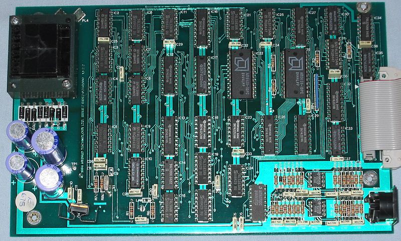
A typical circuit board can have hundreds of components mounted on it. Image by Chris Whytehead — Chris’s Acorns. Licensed underCC BY-SA 3.0, viaWikimedia Commons.

The actual thermal analysis of the circuit board is quite straightforward from the point of view of the analysis itself. Setting up the model in the graphical user interface for COMSOL Multiphysics, however, requires adding many differentBlockandCylinderprimitives and defining their sizes and locations. You also need to define a different dissipation within each device. This can quickly become tedious if you have to do everything by hand.

Now suppose that you’ve been given all of the component types, heat dissipation, locations, and sizes in a spreadsheet.

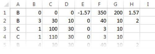
A spreadsheet containing component layout information.

Each row of the spreadsheet represents a different component. This format is very compact and a bit cryptic, so let’s go through what the data means, column-by-column.

The first column can contain a letter, eitherBorC, denoting that the component can be modeled as either aBlockor aCylinderprimitive. The next column is the total heat dissipation within the component (measured in watts). The next three columns represent the location of the component in the global Cartesian coordinate system (measured in millimeters). Lastly, if the row contains a block component, there are three more columns that denote the width, depth, and height of the block. If the row contains a cylinder component, then there are two more columns that contain the radius and height information, respectively.

For the example shown above, the first row of the spreadsheet represents the circuit board itself, which is 1.57 mm thick and 350 mm x 200 mm. It is offset from the origin by -1.57 mm in thez-direction and does not dissipate any heat.

We can write the data in the spreadsheet out to a comma-delimited text file. Let’s now look at how we can read this text file into COMSOL Multiphysics using a simplified app.

Implementing a Simulation App to Read in Model Data

The development of our app begins with a blank model file where we define a3D Componentwith aGeometrythat is tagged asgeom1. These are all default settings. Additionally, we change the unit system in our geometry branch to millimeters, as illustrated in the following screenshot.

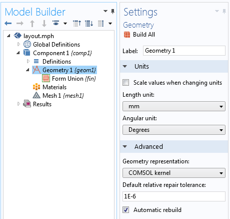
The blank model file within which we build our app. The unit for geometry length is millimeters.

To develop the app itself, we switch over to the Application Builder, which contains the graphical user interface layout and the logic behind our app. The app that will process our text file features a very simple user interface with just four elements:

• File Importfeature
• Graphicswindow
• Filemenu
• Savefeature

The Save feature, found within the File menu, enables us to save our imported data back to a COMSOL Multiphysics file.

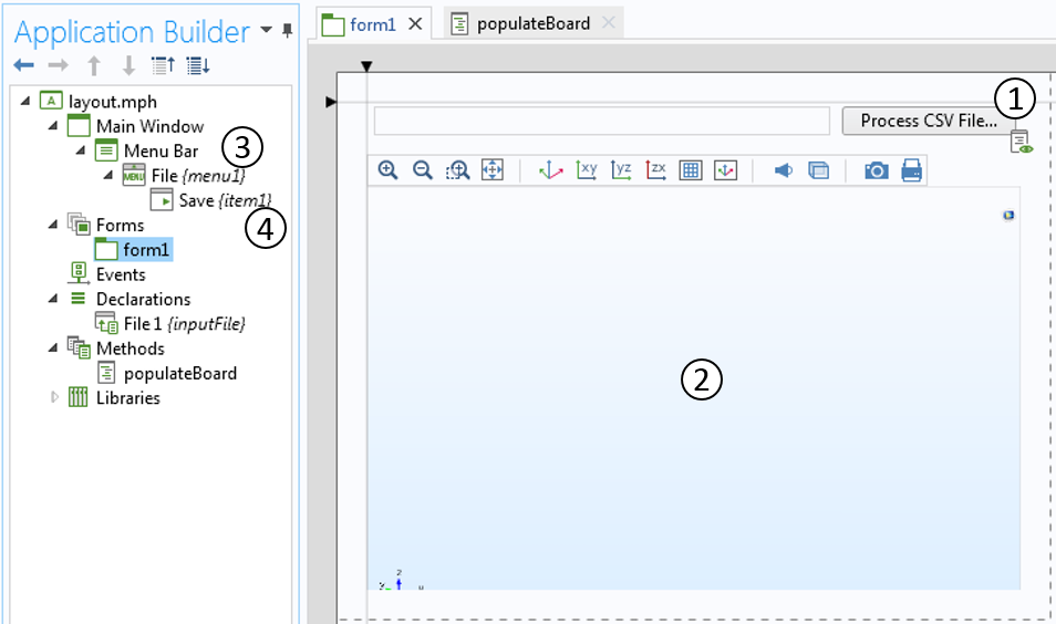
Our app includes a File Import feature, a Graphics window, and a File menu with a Save feature.

In the above screenshot, note that there are two other nongraphic elements included in our app. The first of these elements is aDeclaration, a data structure that is used to store the file name that we are importing. The second element is a method calledpopulateBoard, which processes the text file.

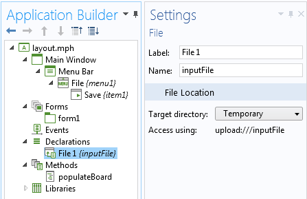
The Declaration settings define how to access the text file.

The one graphical element that the user can interact with here is the File Import feature. The screenshot below highlights the settings for the feature, three of which are important. First, theFile typeshave been set toCSV File, meaning that we can only import comma-delimited files into our app. Second, theFile Destinationis set to theinputFiledeclaration, thus passing the name of the file into this data structure. Finally, when there is a data change (when a different file is selected), thepopulateBoardmethod is called upon.

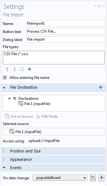
The settings for the File Import feature specify the file type and the method to call upon after a file is imported.

The last part of our app that we need to look at is the method that converts the text file into a COMSOL Multiphysics model. This method is illustrated below, with line numbers added on the left and text strings highlighted in red:

1 String[][] D = readCSVFile("upload:///inputFile"); 2 model.geom("geom1").feature().clear(); 3 for (int k = 0; k < D.length; k++) { 4 if (D[k][0].equals("B")) { 5 model.geom("geom1").create("P"+k,"Block").set("pos", new String[]{D[k][2], D[k][3], D[k][4]}); 6 model.geom("geom1").feature("P"+k).set("size", new String[]{D[k][5], D[k][6], D[k][7]}); 7 } 8 if (D[k][0].equals("C")) { 9 model.geom("geom1").create("P"+k,"Cylinder").set("pos", new String[]{D[k][2], D[k][3], D[k][4]}); 10 model.geom("geom1").feature("P"+k).set("r", D[k][5]); 11 model.geom("geom1").feature("P"+k).set("h", D[k][6]); 12 } 13 model.geom("geom1").feature("P"+k).set("selresult","on"); 14 model.variable().remove("var"+k); 15 model.variable().create("var"+k).model("comp1"); 16 model.variable("var"+k).selection().named("geom1_P"+k+"_dom"); 17 model.variable("var"+k).set("Q", D[k][1]); 18 } 19 model.geom("geom1").run();

Now we’ll go through the method line-by-line:

1. Read the data from the CSV file, accessing the filename as defined by the declaration.
2. Clear out the existing geometry sequence in the file (necessary if we want to read in a different CSV file).
3. Set up a for loop over all of the lines (rows) in our CSV file.
4. If the first entry on the line is the text string “B”, then we are defining a block.
5. Create a new block primitive, located at thexyz-position and specified by columns 3-5 of the CSV file.
6. Set the size of this block primitive to the dimensions specified by columns 6-8 of the CSV file.
7. Close the “if” statement for the block creation.
8. If the first entry on the line is the text string “C”, then we are defining a cylinder.
9. Create a new cylinder primitive, located at thexyz-position and specified by columns 3-5 of the CSV file.
10. Set the radius of the cylinder.
11. Set the cylinder height.
12. Close the “if” statement for cylinder creation.
13. Create a selection out of the feature that was just created. Regardless of the type, it will have a tag identifier of “Pk”, where k is the integer index.
14. Remove any defined variables that exist with conflicting names.
15. Create a new variable with an “s” name based upon the integer index.
16. Apply the newly created variable to the selection corresponding to the new part.
17. Define a variable “Q” that is the dissipation in this part, specified by column 2 of the CSV file.
18. Close the for loop over the input file.
19. Finalize the geometry.

So, in just under twenty lines of code, we have converted a text file into a COMSOL Multiphysics model! And that’s all there is to our app. Of course, this code assumes that our input file is error free and doesn’t contain any invalid data or unrecognized characters. We could extend this code to be fault tolerant and to do some sanity checking, such as making sure there are no overlapping parts, if desired.

Let’s now take a look at the results we would obtain with some sample input…

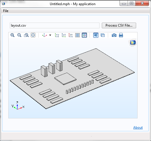
The graphical user interface of our app after reading in a sample CSV file.

We can also write out a full COMSOL Multiphysics file from this app. The file will contain all of the geometry as well as all of the heat loads in each part, defined as variables. You could then perform the thermal analysis in COMSOL Multiphysics, or you could extend the current app to perform a thermal analysis of the entire board within the app itself. You will, of course, still need some boundary conditions and you will need to define material properties in all of the components. Hopefully, however, it is clear by now that you have the ability to extend the app to read such information in from the same CSV file.

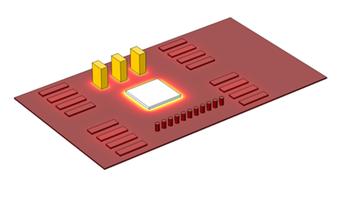
Once all of the part geometries and different heat loads are defined within a COMSOL Multiphysics model, you can compute the temperature distribution on the circuit board.

Additional Resources for Designing Apps and Thermally Analyzing Circuit Boards

• Want to build this app yourself but haven’t used the Application Builder yet? Here are some resources to get you started:
  • Download theIntroduction to Application Buildermanual
  • Watch videos designed to help you learn about and use theApplication Builder and COMSOL Server™
  • Browse our blog posts to see how simulation apps are applied to arange of applications
• Interested in learning more about the thermal analysis of circuit boards? Try out these tutorials from our Application Gallery:
  • Disk-Stack Heat Sink
  • Convection Cooling of Circuit Boards — 3D Natural Convection
• Seeking more information on how to build a specific type of app or have other modeling inquiries?Contact us