

In the Semiconductor Module, as of version 5.6 of the COMSOL Multiphysics® software, we have expanded the capability of theSchrödinger Equationphysics interface from single-component to multiple-component wave functions. This allows the simulation of a wider range of systems, such as particles with spins and the valence band structure with a mixing of the 3 p-like orbitals. In this blog post, we use a simple benchmark model to illustrate how to use this multicomponent wave function functionality.
The Hamiltonian Matrix
When the wave function has more than one component, the Hamiltonian becomes a matrix to operate on the vector of the wave function components. For example, the time-dependent Schrödinger equation now reads
(1)
whereNis the number of wave function components.
The minus sign on the right-hand side of the equation for the time evolution operator is due to the fact that all physics interfaces in COMSOL Multiphysics take the engineering sign convention ofexp(-i k x + i \omega t)instead of the physics sign convention ofexp(i k x – i \omega t). Later on, we will see that the sign of the momentum operator also differs from the one seen in most textbooks because of this.
In general, each element of the Hamiltonian matrix\mathbf{H}_{mn}can include several terms of zero, one, or two partial derivatives:
(2)
\frac{+\hbar^2}{2\,m_e} \sum_{ i,j\in \{1,2,3\}} \left[
\frac{i\, \partial}{\partial r_i} \,A_{ij}^{mn}(\mathbf{r}) \, \frac{i\, \partial}{\partial r_j}
+ \frac{i\, \partial}{\partial r_i} \,H_i^{mn(1R)}(\mathbf{r})
+ H_j^{mn(1L)}(\mathbf{r}) \, \frac{i\, \partial}{\partial r_j}
+ H^{mn(0)}(\mathbf{r})
\right]
wherem_eis the electron mass;\mathbf{r}is the position vector\mathbf{r}=\{r_1,r_2,r_3\}\equiv\{x,y,z\}; andA,H^{(1R)},H^{(1L)}, andH^{(0)}are coefficients that may be spatially varying.
In the first term, the differential operator on the left is understood to act on both the coefficientAand the wave function component\psi_{n}. Similarly, the differential operator in the second term acts on bothH^{(1R)}and\psi_{n}. Note that all of the momentum operators differ by a minus sign from the usual convention, as discussed earlier.
The number of elements of the Hamiltonian matrix grows as the square of the number of wave function components. Each element may contain terms of various orders of partial derivatives, as shown inEq. 2. To provide flexible and efficient ways to enter these terms into the graphical user interface within the limited window size, we have created a number of built-in features as of version 5.6. In the example model below, we show how to use these features.
The Model System
As mentioned above, all of the coefficients in the Hamiltonian matrix elements can be spatially varying. This is particularly true in heterostructures and nanostructures, such as quantum wires and quantum dots. For simplicity, we have chosen a model of a uniformly strained bulk crystal, where all coefficients are spatially uniform. Nevertheless, this simple model still serves the purpose of illustrating the procedure to enter the Hamiltonian matrix elements into the user interface. In addition, it also serves as a benchmark model to verify the numerical solution with the analytic solution of this simple system.
Gallium nitride (GaN) is an important wide band gap semiconductor material for optoelectronics, high-power, and high-frequency applications. Chuang and Chang published their derivation and computation of the 6-by-6 Hamiltonian matrix for wurtzite crystals including GaN in 1996 (Ref. 1). In Eq. 45 of the paper, the 6-by-6 Hamiltonian matrix is block diagonalized, and the upper left 3-by-3 matrix reads
(3)
F & K_t & -i H_t \\
K_t & G & \Delta-i H_t \\
i H_t & \Delta+i H_t & \lambda
\end{array}\right]
The matrix elements are given by Eqs. (34) and (42) inRef. 1. For example, the element at the (1,1) position of the 3-by-3 Hamiltonian matrix is
(4)
The first two terms are numbers and the other two contain operators and numbers:
(5)
(6)
To compare with the result shown in Fig. 5 in the paper, we will set they-component of the crystal momentumk_yto zero. For theSchrödinger Equationinterface, the other two components,k_xandk_z, are replaced by the partial derivativesi\partial / \partial xandi\partial / \partial z, respectively (see footnote). So, the two equations above become
(7)
i\frac{\partial}{\partial z} A_1 i\frac{\partial}{\partial z}
+ i\frac{\partial}{\partial x} A_2 i\frac{\partial}{\partial x}
\right]+\lambda_\epsilon
(8)
i\frac{\partial}{\partial z} A_3 i\frac{\partial}{\partial z}
+ i\frac{\partial}{\partial x} A_4 i\frac{\partial}{\partial x}
\right]+\theta_\epsilon
Finally, the numbers contributed from the strain are
(9)
(10)
where\epsilonis the strain components.
The energy parameters\Delta_1and\Delta_2, the effective mass parametersA_1~A_1, and the deformation potentialsD_1~D_1are listed in Table III ofRef. 1.
Expanding outEq. 4for the elementFat the (1,1) position of the 3-by-3 Hamiltonian matrix, usingEq. 7and8, we get
(11)
\frac{\hbar^2}{2m_e}\left[
i\frac{\partial}{\partial z} (A_1+A_3) i\frac{\partial}{\partial z}
+ i\frac{\partial}{\partial x} (A_2+A_4) i\frac{\partial}{\partial x}
\right]
+\Delta_1+\Delta_2
+\lambda_\epsilon
+\theta_\epsilon
We have collected the operators in the first term, and the other four terms are numbers.
Numerical and Analytic Methods
In Fig. 5 ofRef. 1, the valence band dispersions along thek_xandk_zdirections are plotted for unstrained and strained crystals, withk_yset to zero. Since the systems under consideration are bulk crystals,k_xandk_zare just numbers, and the Hamiltonian(3)reduces to a 3×3 matrix of certain numerical values corresponding to the given values ofk_xandk_z. The eigenvalues of this matrix can be computed numerically to obtain the band structure shown in the figure. This is the analytic approach taken by the paper and will be used to verify the numerical approach to be discussed next.
In a general nonuniform structure, such as quantum wells and quantum dots, the numbersk_xandk_zhave to be replaced by the partial derivativesi\partial / \partial xandi\partial / \partial z, as mentioned earlier, and the Schrödinger equation on thexz-plane is solved to obtain the band structure. This is the numerical approach. Of course, this becomes overkill for the simple system of a bulk crystal. However, for the purpose of teaching and verification, we have chosen this simple system. Once you have learned how to use the physics features to build this simple model, you are equipped to simulate more complex systems solvable only by the numerical approach.
The COMSOL Multiphysics® Model
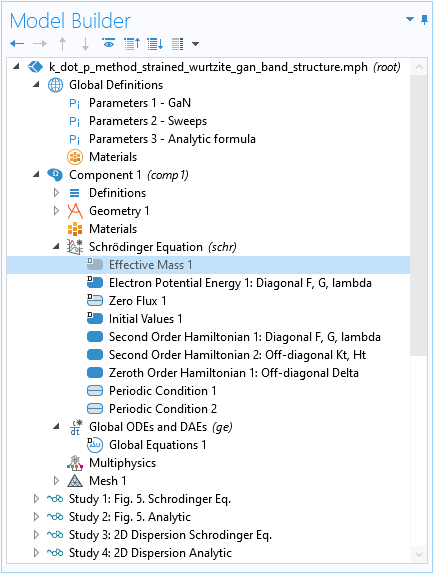
It is straightforward to set the number of wave function components to 3 in either the Model Wizard or the physics interfaceSettingswindow, since the size of the Hamiltonian is 3×3.
The model is 2D in thex– andzdirections, as discussed above. To make the model notation easier to read, we change the coordinate name for the second axis from the defaultytoz, as shown in the screenshot below.
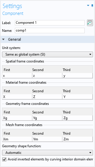
Change the coordinate names to match the directions of interest (xandz).
Since we are only interested in the band structure near the zone center, we can use a simple square domain slightly smaller than the unit cell, and use the Floquet–Bloch periodic boundary conditions for the Schrödinger equation. In this regime, the problem approaches a uniform continuum and a small number of mesh elements is sufficient. (See thetutorial model of a thin-film BAW structurefor a mechanical model using the same technique.)
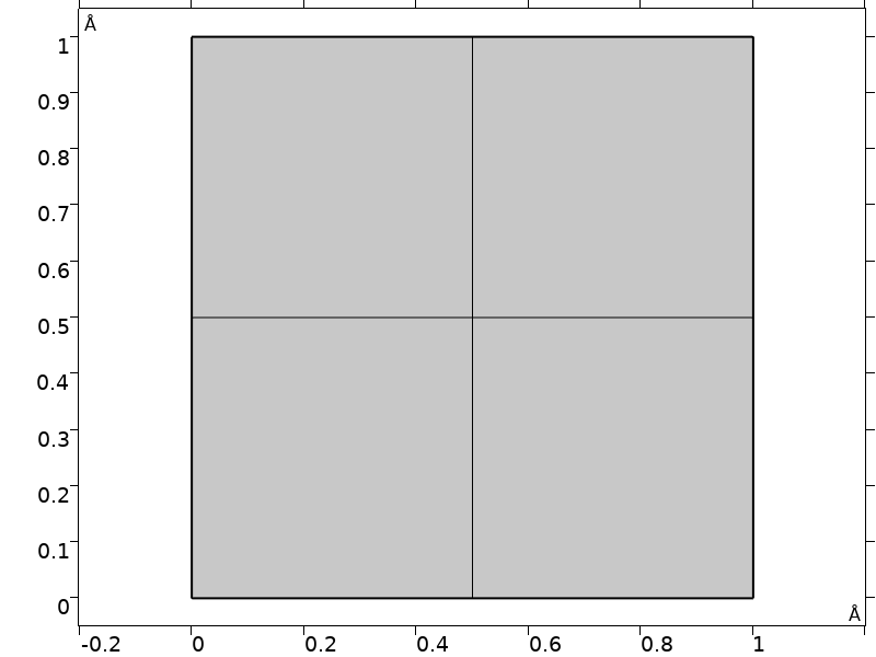
Domain and mesh used in the model.
To conveniently create a plot to compare with Fig. 5 in the paper, we set up a swept parameterkp, such that its positive axis represents thekx-axis and the negative axis represents thekz-axis. Use the if statement in the expressions for the parameterskxandkzto achieve this, as shown in the screenshot below.
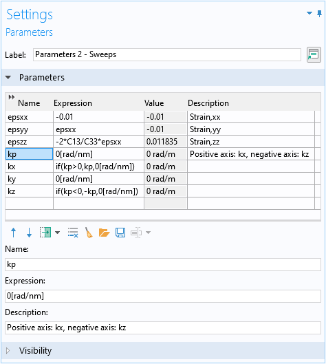
Set up a parameterkpfor the dual axis 1D plot forkxandkz.
Analytic Solution
For the analytic approach, we set up a global equation to diagonalize the 3×3 Hermitian matrix given byEq. 3. We use the reserved namelambdafor the eigenvalue in the global equation. We scale the Hamiltonian with the energy scale of 1 meV so that the source term is about the order of unity, and the eigenenergy is the eigenvalue in the unit of meV. We also add some blank spaces in the expressions to align the columns of the matrix.
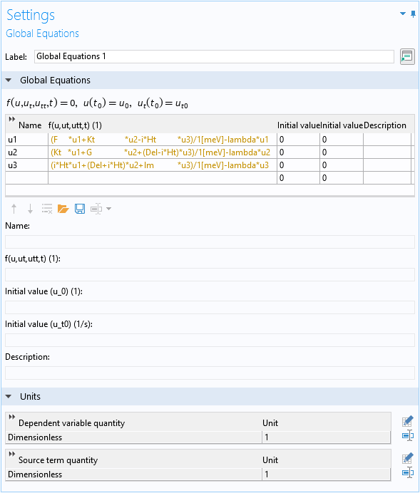
Global equation to find the eigenvalues of the 3×3 matrix.
The text is yellow because at this point, the eigenvalue variablelambdais not yet defined.
Solving the Schrödinger Equation
As mentioned earlier, the numerical approach solves the Schrödinger equation. To conveniently create a plot to compare with Fig. 5 in the paper, we set theEigenvalue scaleto the same energy unit as the vertical axis of the figure (meV), so that the eigenvalue takes on the numerical value of the eigenenergy in the same unit (meV).
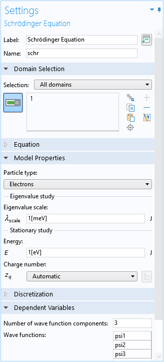
Settings window of theSchrödinger Equationphysics interface.
Hamiltonian Matrix Input
Now, we are ready to enter the matrix elements of the 3×3 Hamiltonian. Again, we use the elementFat the (1,1) position as an example. The contributions to this element are summarized inEq. 11. The first term contains second-order derivatives, so we add aSecond Order Hamiltoniandomain condition. This feature was introduced as of COMSOL Multiphysics 5.6, together with the capability of handling multiple-component wave functions for theSchrödinger Equationphysics interface.
The central feature in theSettingswindow for this domain condition is theHamiltonian input table. The first two columns of this table are for the row and column indices of the Hamiltonian matrix element to be entered. Each index is selected from a drop-down menu, which is automatically populated from 1 toN(the number of wave function components). For example, here we have setNto 3, so the drop-down menu has the choices of 1, 2, or 3. Always decide on and set the number of wave function components before you start entering data into the table (see the sectionKnown Limitationbelow).
The third and fifth columns are for the two differential operators. They are also provided as drop-down menus with automatic population of differential operators according to the spatial dimension of the model. Here, we have set up a 2D model on thexz-plane, so the choices arei\partial / \partial xandi\partial / \partial z.
The fourth column is for the effective mass parameterA. As with almost all other input fields in COMSOL Multiphysics, the input field accepts a number, parameter, variable, or any other mathematical formula. A prefactor of\hbar^2/2m_eis always built in for this type of domain condition, including the current one,First Order Hamiltonian, Left,First Order Hamiltonian, Right, andZeroth Order Hamiltonian.
The last column,Description, gives us an opportunity to document each entry in the input table. Each element in the Hamiltonian matrix, for example, the elementFgiven byEq. 11, contains different types of terms, which will be entered into multiple table rows across several different features. As such, it is important to keep track of each table row by entering appropriate comments in theDescriptioncolumn.
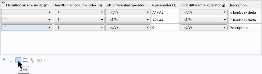
The screenshot below shows theSettingswindow of the domain condition, with the first term inEq. 11entered into the first two rows of theHamiltonian input table. The position of the matrix elementFis (1,1), so both the row and column indices are 1. The differential operators and the A parameters of the two rows in the table correspond to the two terms in the square brackets inEq. 11. TheDescriptioncolumn records the source of the contribution; in this case, the two rows come from theF=\lambda+\thetapart ofEq. 4originally.
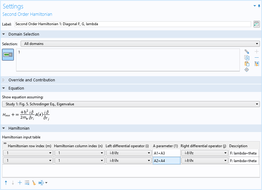
The settings window for theSecond Order Hamiltoniandomain condition, with the first term of the matrix elementFentered.
Copy/Paste Table Rows
Before entering the rest of the terms for the (1,1) elementF, we notice that the second-order operator part of the (2,2) elementGis identical to the one ofF. From Eq. 34 ofRef. 1:
(12)
so we get the same contributions to the second-order Hamiltonian (G=\lambda+\theta), except the position is different: instead of (1,1), now it’s (2,2).
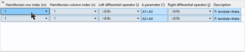
Instead of filling in two more rows of data forGfrom scratch, we can copy and paste the two rows forFand just change the row and column indices to 2. First, click and drag the mouse to select the two rows in the table:
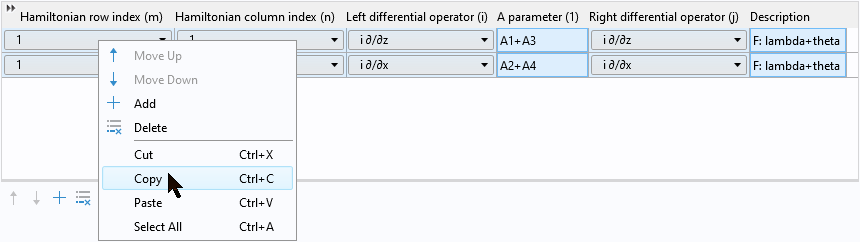
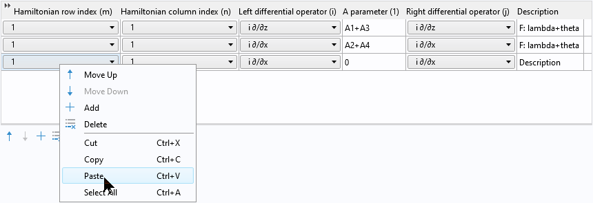
Then right-click to copy the selected rows:
Then click the Add button to add a new row:
Then right-click to paste the two copied rows into the table:
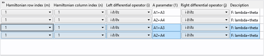
After pasting, we have two pairs of identical rows:
Finally, change the row and column indices from 1 to 2 and update the description:
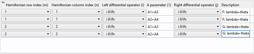
Reusing table rows in this way not only saves time but also helps avoid mistakes!
Disable Default Effective Mass Contribution
TheSecond Order Hamiltoniandomain condition that we just demonstrated for the diagonal elements corresponds to the kinetic energy terms normally added by the defaultEffective Massfeature. We should disable it to remove the unwanted default contribution to the Hamiltonian.
Disable the defaultEffective Massfeature to remove its unwanted contribution to the Hamiltonian.
Terms Without Operators
To enter the rest of the terms for the (1,1) elementF(last 4 terms inEq. 11:\Delta_1+\Delta_2+\lambda_\epsilon+\theta_\epsilon), which are just numbers, we can use either theZeroth Order Hamiltoniandomain condition, or the defaultElectron Potential Energydomain condition, as shown in the screenshot below, since the element is on the diagonal of the Hamiltonian matrix.
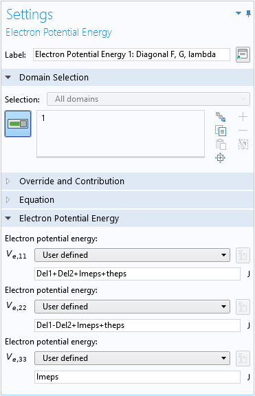
Use the defaultElectron Potential Energydomain condition for the zeroth-order terms of the diagonal elements of the Hamiltonian matrix.
Off-Diagonal Elements
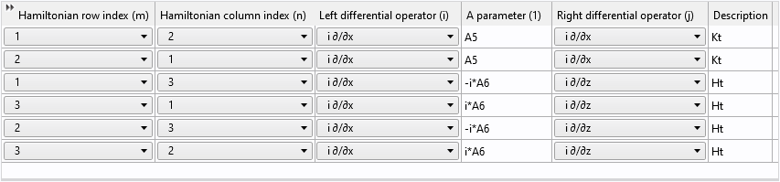
For the off-diagonal elements, we follow the same procedure to fill in the Hamiltonian input table for the second-order terms:
And the zeroth-order terms:
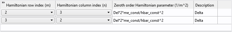
As mentioned earlier, theZeroth Order Hamiltonianhas the prefactor of\hbar^2/2m_ebuilt in; therefore, if the input quantity (Delin this case) is an energy unit, it needs to be divided by the prefactor.
Known Limitation
If the number of wave function components is changed after a Hamiltonian matrix input table has been filled with data, the table rows will become out of sync. At this point, the table needs to be cleared and filled with data again. We recommend that you first determine the particular Hamiltonian matrix that you would like to study in a model and enter the number of wave function components accordingly, before filling any Hamiltonian input table with data.
Other Settings
It is straightforward to set up the Floquet–Bloch periodic boundary conditions to create the simple mapped mesh and configure sweeps of the wave vectors using the specially prepared parameterkpin the eigenvalue studies.
To solve the analytic 3×3 matrix equation configured with the global equation, use theAlleigenvalue option to obtain all 3 eigenvalues of the 3×3 matrix equation.
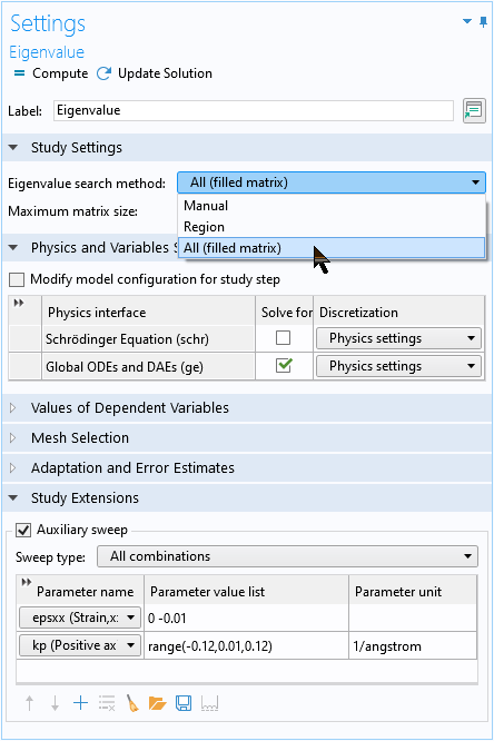
Use theAlleigenvalue option to obtain all 3 eigenvalues of the global equation.
Computed Band Structure for Unstrained and Strained Wurtzite Crystals
The two figures below show the computed unstrained and strained heavy hole (HH), light hole (LH), and crystal-field split-off hole (CH) dispersions along the positivekx-axis and negativekz-axis directions, agreeing well with analytic solution (circles) and Fig. 5 inRef. 1.
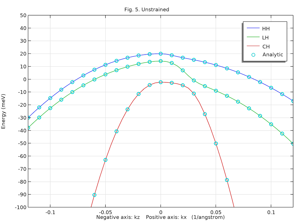
Unstrained valence band structure of the bulk GaN wurtzite crystal.
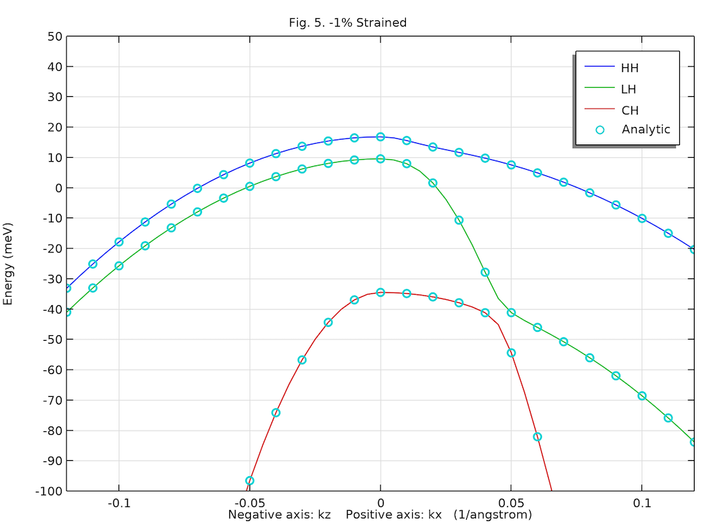
Compressively strained valence band structure of the bulk GaN wurtzite crystal.
The plot below compares the 2D energy surfaces along thex– andzdirections for the 3 valence bands between computed values (color surface) and the analytic solution (gray wireframe). The agreement is also very good.
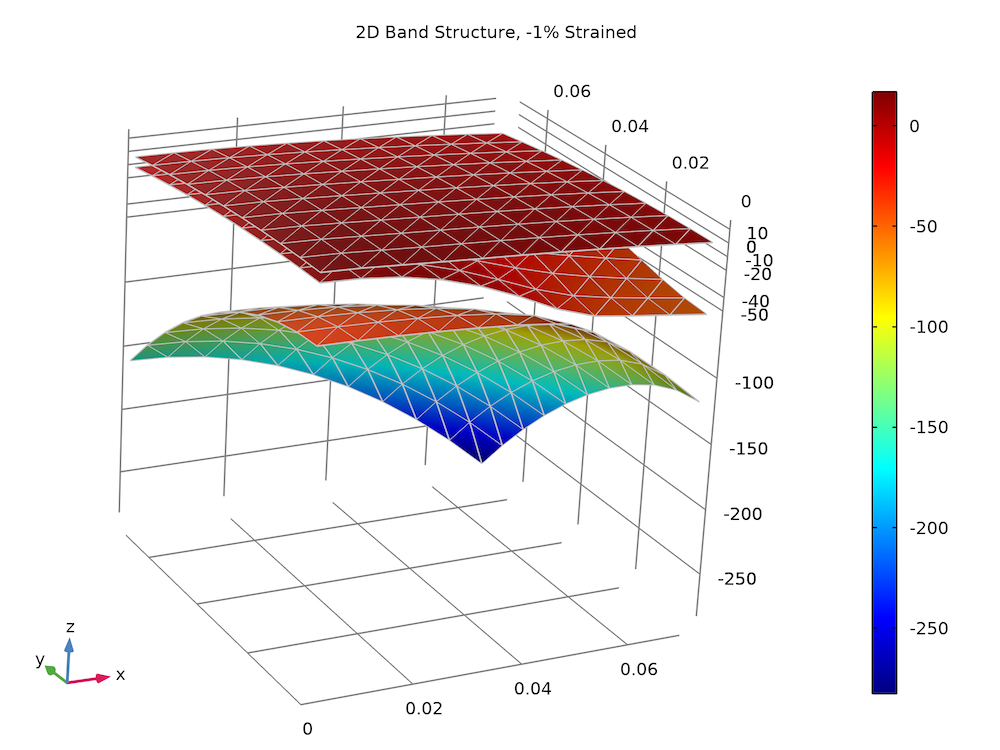
Strained valence band structure of the bulk GaN wurtzite crystal.
Conclusion
In this blog post, we demonstrated the new capability of theSchrödinger Equationphysics interface to handle multicomponent wave functions, using a simple bulk crystal example. The Hamiltonian matrix is systematically entered into the user interface with built-in features. The same methodology can be applied to more complex systems, such as quantum wells and quantum dots. We would love to hear about how you use this new capability for your simulation projects!
Try It Yourself
Try modeling a strained wurtzite GaN band structure yourself by clicking the button below, which will take you to the Application Gallery and a downloadable MPH-file:
Reference
- S.L. Chuang and C.S. Chang, “k·p method for strained wurtzite semiconductors,”Phys. Rev.B, vol. 54, p. 2491, 1996.
Footnote
Recall that COMSOL’s sign convention for the time harmonic phasor isexp(+i \omega t), so a plane wave isexp(+i \omega t-i k_x x). Thus the operator+i\partial / \partial x, not-i\partial / \partial x, is used.

Comments (7)
Nikhil Sen
November 11, 2021Hi Chien
Thanks for excellent blogpost. It helped me a lot to learn the COMSOL, specifically Schrodinger equation solver.
I was wondering how does the eigenvalue problem is solved with kp as the sweeping parameter? I am asking this question because I see no explicit mention of kx or ky terms in the Hamiltonian matrix.
Chien Liu
November 11, 2021 COMSOL EmployeeThank you Nikhil for the comment! You are right that kx and kz does not appear explicitly in the Hamiltonian but they are used in the Floquet–Bloch periodic boundary condition. Hope this helps. Sincerely, Chien
Nikhil Sen
November 11, 2021Thanks Chien for prompt reply. And it does answer my previous question.
I have an additional question, when I use kp as one of the k-vector for the Floquet-Bloch periodicity, I get separate data points (eigne values) in the graph as opposed to continuous line. Additionally, I also get legend for every value of kp (& corresponding eigen energy) in the graph rather than for the entire band (e.g. HH, LH etc). Why does this happen?
Is it something to do with how kx and kz are defined that we don’t get legend for every eigen value when k-vector for the Floquet-Bloch periodicity are kx and ky?
Thanks again for your help.
Nikhil Sen
November 11, 2021I did a little deeper digging and I found that kx and kz are defined when the Floquet-Bloch periodic condition is applied.
Does it mean that what is kx and kz is defined when the Floquet Bloch condition is defined (at least in this specific example?
Chien Liu
November 11, 2021 COMSOL EmployeeLooks like our messages crossed but yes as I said above kx and kz are used in the Floquet–Bloch periodic boundary condition. Hope this helps. Sincerely, Chien
Nikhil Sen
November 11, 2021Hi Chein
Sorry for confusion. I think there is a slight confusion.
My previous question was answered but my new question is this:
I have an additional question, when I use kp as one of the k-vector for the Floquet-Bloch periodicity, I get separate data points (eigne values) in the graph as opposed to continuous line. Additionally, I also get legend for every value of kp (& corresponding eigen energy) in the graph rather than for the entire band (e.g. HH, LH etc). Why does this happen?
Is it something to do with how kx and kz are defined (in parameter-sweep) that we don’t get legend for every eigen value when k-vector for the Floquet-Bloch periodicity are kx and ky?
Thanks again for your help.
Chien Liu
November 11, 2021 COMSOL EmployeeHi Nikhil, If you follow the step-by-step instructions in the PDF documentation accompanying the example model, you should be able to generate the same plots. If you need further assistance, please do not hesitate to contact us atsupport@comsol.com. Sincerely, Chien