Probing Your Simulation Results

For a transient simulation, imagine if you could simply insert a virtual sensor in a model at a certain location and then monitor the evolution of a field value over time while solving. In COMSOL Multiphysics^®you can do just that by usingProbes. You define a probe in theModel Buildertree right under theModel Definitionsnode. Measuring the value at a point is not the only thing you can do with probes, but in this blog post we will focus on that specific task of probing. We’ll also show you how you can use probes to compress the size of a saved transient model by only storing the full solution data set at a few points in time and at the same time having a densely sampled probe data plot with an accompanying table.

Probing a Fuel Cell Bipolar Plate Simulation

To better illustrate probing, let’s use an example. We’ll show you how to use probes in the case of a transientthermal stressanalysis. (Tip: Read our previous blog post for some background onthermal stress analysis.)

Let’s analyze a bipolar plate of a proton exchange membrane fuel cell (PEMFC). The geometry of this model is taken from theModel Libraryof theStructural Mechanics Module. The PEMFC is a candidate technology for future hydrogen-powered vehicles, but the very expensive materials needed have so far limited its use to high-cost applications, such as certain space missions. Fuel cell simulations contribute to designing less expensive fuel cells and making this technology more widely available. Fuel cell design requires extensive multiphysics simulations including stress, heat, CFD, and electrochemical analysis. We won’t look at a CFD and electrochemical analysis here, but instead show you a mechanical simulation. If you are interested in more advanced fuel cell simulations, check out thetutorial models of the Battery Design Module.

About the Fuel Cell Bipolar Plate Model

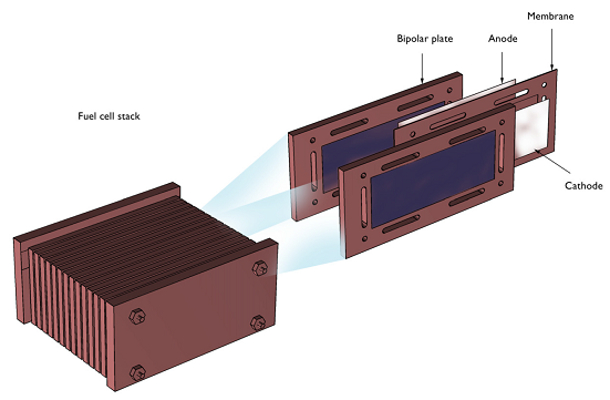
A fuel cell stack consists of unit cells with an anode, a membrane, and a cathode connected in a series through bipolar plates. The bipolar plates also serve as gas distributors for hydrogen and air that is fed to the anode and cathode compartments, respectively. The picture below shows a schematic drawing of a fuel cell stack. The unit cell and the surrounding bipolar plates are shown in detail in the upper-right corner of the figure.

The fuel cell operates at temperatures just below 100°C (212°F), which means that it has to be heated at start-up. The heating process induces thermal stresses in the bipolar plates. The figure below shows the detailed model geometry. The plate consists of gas slits that form the gas channels in the cell, holes for the tie rods that keep the stack together, and the heating elements (in the picture labeledHeat source), which are positioned in the middle of the gas feeding channel for the electrodes.

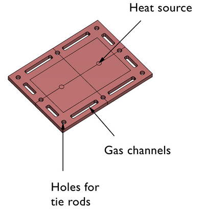
In the COMSOL model of the bipolar plate, we use theThermal Stressuser interface and apply a volume heat source to the two central cylindrical domains.

There are also convective cooling boundary conditions applied to the sides of the plate.

A total power of 8 W is distributed over the two heating elements. We’ll ramp up the heat power by defining a look-up table that we namestartup(), withtimeas input argument. The bracket notation with 1/s (see image below) converts the input argument t to a unitless quantity before being passed to the look-up table. This unit conversion is not required but it is a good practice to take charge over the unit handling.

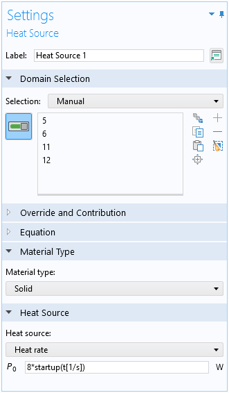
The interpolation table is defined underModel Definitionsand represents an increase from 0 to 1 over 10 seconds. We use thePiecewisecubic interpolation option to make sure we get a smooth curve. This curve will modulate the input power of 8 W over time so that at t=0 s the input power is 0 W and at t=10 s the input power is the final 8 W. We’ll see below that the time for the bipolar plate to reach steady-state is much longer than 10 seconds due to the relatively inefficient cooling:

How to Set up Probes in COMSOL Multiphysics^®

Setting up probes is done from theModel Definitionsnode in theModel Treeof the COMSOL Desktop^®. In this case we’ll choose aDomain Point Probe(there are several other types of probes). By using thePoint and surface normalLine entry methodwe get to interactively pick a point on a line that goes from another point on the model boundary with direction normal to the surface of the boundary. The depth can very easily be fine-tuned by the slider control. You also get the exact position of the point in x, y, and z coordinates.

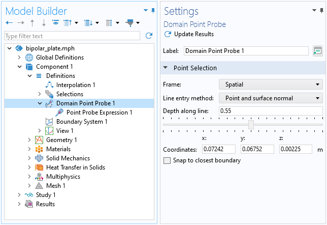
The probe location is indicated with a red dot along the line. Here, an arbitrary point is picked on the inside of the plate:

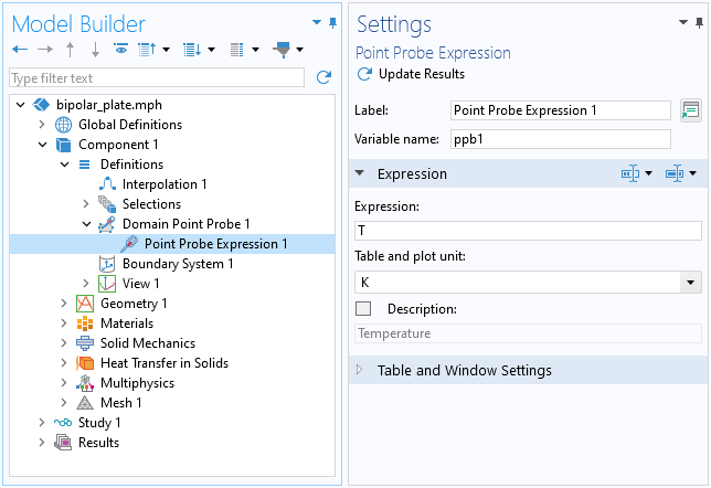
Underneath theDomain Point Probenode in theModel Buildertree you will find a node calledPoint Probe Expression. Here you can set the field variable you wish to evaluate for and monitor during the solution process. The default for thermal stress analysis is the temperature field T but this could really be any field expression you’d like to monitor, including gradient (partial derivative) components. For example, the partial derivative of T with respect to X would be entered as d(T,X) or simply TX (notice the capital X).

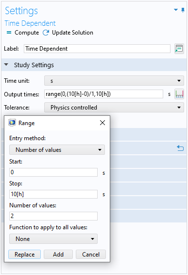
In theStudy Settingswindow, we can use theRangetool to specify a start and stop time. Units can be used here and we’ll solve for 10 hours, entered as 10[h].

Avoid Storing the Entire Solution with Probing

Now let’s see how probes can be used to avoid storing the entire solution for a large number of time steps. In theRangetool we set theNumber of valuesto 2. This is the smallest possible value and will make sure to only store the full solution at t=0 and t=10[h]. The accuracy of the time-dependent solver is controlled by theRelative tolerance. In this case, the tolerance is lowered from the original 0.01 to 0.0001 (see image above). The lower the tolerance, the shorter the time-steps taken by the solver. This will have an impact on our probe data. We can set the probe to be updated at the same time steps as taken internally by the solver. (The time-stepping algorithm used by COMSOL^®for this simulation is a so-called variable-order BDF method that adapts its steps in time, based on the solution and the tolerance settings.)

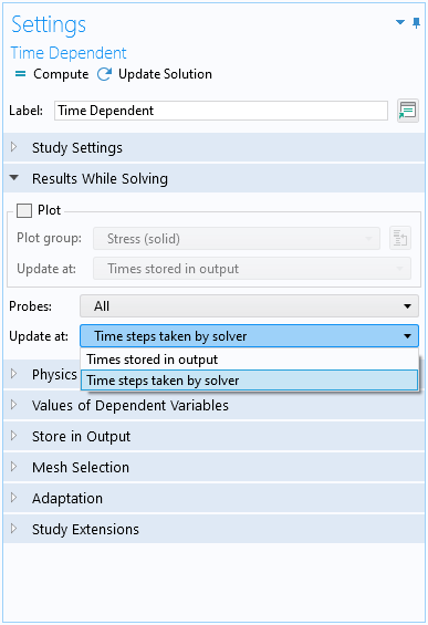
In theStudy Settingswindow, in the section calledResults While Solving, we change from theOutput from solveroption (which would just give us the results at t=0 and t=10[h]) toSteps taken by solver. Like this:

SelectComputefrom theStudynode. During the solution, we’ll now see aProbe PlotandProbe Tableof theTemperaturewhile the solver is working. If you have a simulation that takes a long time to solve, you can use the displayedProbeinformation to check if you set something up wrong in the model. Doing so allows you to then stop the simulation before it’s finished, go back and change some settings, and start over again.

As you can see, the probe output has many more data points in time than just t=0 and t=10[h]. By lowering the solver tolerance setting you can increase the number of data points. The table allows you to copy-and-paste the results for use in a spreadsheet. You can also change the settings of theProbe Plotif you wish to use different units or ordering of the axes (here we get temperature T vs. time t).

Visualizing our Results

As a next step we can of course also visualize the Temperature field at 10 hours (36,000 s) as well as the von Mises Stress with an overlaid mesh plot.

Visualization of Temperature field at 10 hours (left). Visualization of von Mises Stress with overlaid mesh (right).

Note: The mesh in this example has prismatic finite elements; triangles swept through the thickness of the plate.

Editor’s note: This blog post was updated on March 4, 2024, to include updated screenshots.