学习中心

Considerations for Detailed Finite Element Analyses

---

Speaker driver design usually requires a full and detailed electrovibroacoustic analysis in order to understand how some key design variables affect the electromagnetic properties, the vibration behavior of the moving parts, and the sound radiation pattern generated. Analysis that includes all of the acting electromagnetic and mechanical components of a driver allows you to understand the linear behavior of the driver; to optimize the dimension, shape, or topology of a specific component in the driver; or to study the nonlinear distortion when deformation becomes large.

To perform electrovibroacoustic analysis in the COMSOL Multiphysics^®software, you need to solve a fully coupled problem that combines the electromagnetic field with structural vibrations and acoustic radiation. The finite element method (FEM) is the most often used approach at this stage, and COMSOL Multiphysics^®has built-in features that couple the physics interfaces for modeling different types of speaker drivers, as described in our blog post “Modeling Speaker Drivers: Which Coupling Feature to Use”. Here, we use a conventional dynamic speaker driver as an example and discuss the important concepts in setting up a multiphysics FEM model for speaker driver analysis.

Background and Introducing the Example

A typical dynamic transducer is composed of a permanent magnet, which is responsible for generating the magnetic field, and a multiturn coil placed within this field. When an AC voltage (current) is applied to the coil, an electromagnetic force — referred to as theLorentz force— is generated. This force induces vibrations in the coil and the connected diaphragm, leading to sound being radiated.

Conversely, the coil's motion within the magnetic field triggers a voltage induction within the coil. This phenomenon, known asback EMF(EMF beingelectromotive force), subsequently influences the magnetic field. This interplay of forces and induced voltages is the foundational mechanism behind conventional dynamic speaker drivers that are based on moving coils.

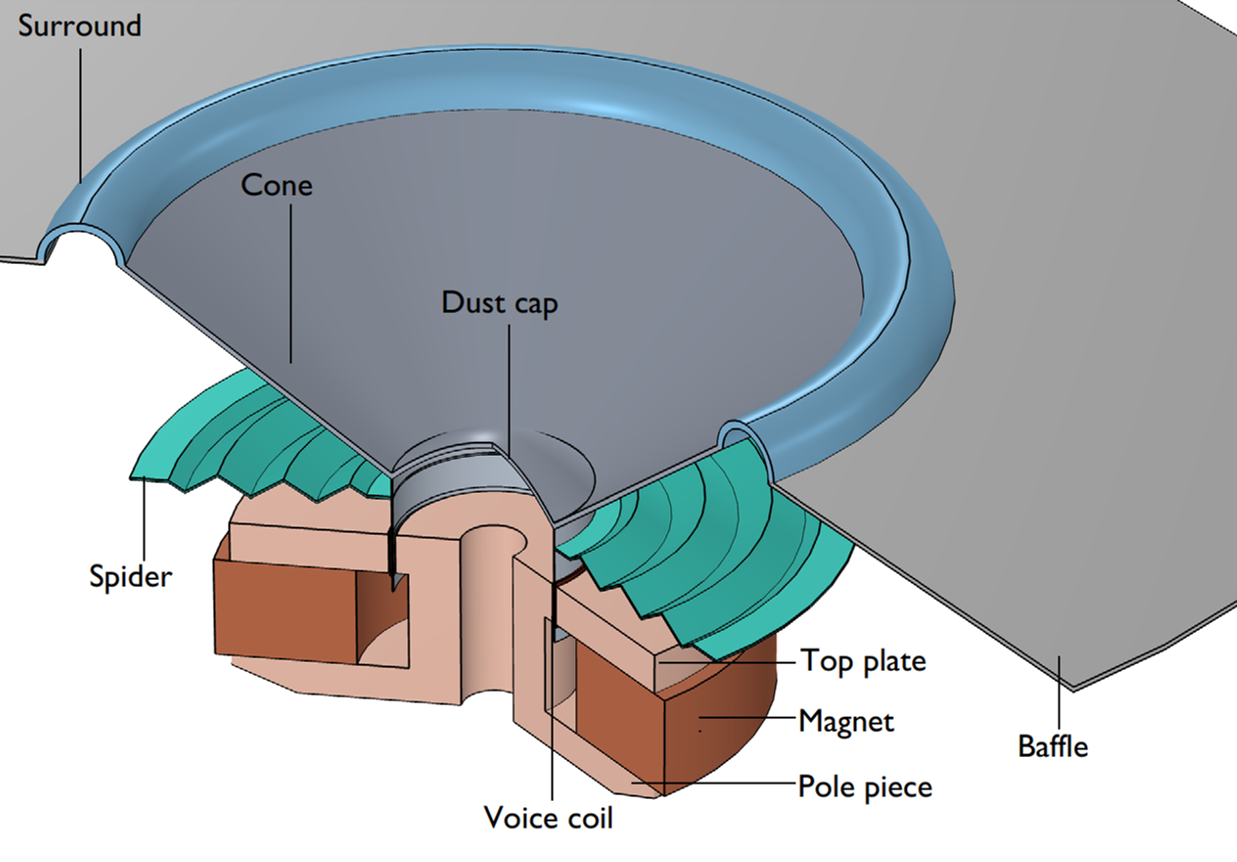A moving coil transducer uses Lorentz force to induce vibration

Solving the Problem in Frequency Domain or Time Domain

The magnetic field in a dynamic transducer includes two components, a static component induced by the permanent magnet and an oscillatory component generated from the AC current in the voice coil. Modeling the contribution from both requires a two-step study: First, aStationarystudy step is necessary for solving the static magnetic field induced by the magnet. This should be followed by a second study step for computing the perturbed solution of all fields around the bias solution computed in the first step.

The second study step can either be aFrequency-Domain, Perturbationstudy or aTime Dependentstudy based on the characteristics of both the excitation and solution. AFrequency-Domain, Perturbationstudy type is applicable under the following conditions:

• The oscillatory excitation is harmonic and continuous
• The magnitude of oscillation is small and the system stays linear
• The output of interest is the steady-state time-harmonic solution
• The study is used for computing the response of a linear or linearized model subjected to harmonic excitation around a bias for one or multiple frequencies.

Should any of these conditions fail to hold, aTime Dependentstudy should be used in the second step. This would be necessary under the following circumstances:

• If the excitation takes the form of a short pulse or includes more than one frequency component.
• If the system introduces a nonlinearity. The nonlinearity can be due to large signal excitation and higher harmonic generation, a nonlinear magnetization model, or geometry change because of large deformation.
• The output of interest is the transient response to an excitation, rather than a steady-state time-harmonic solution.

To create the two-step study, you can first select theStationarystudy type from thePreset Studies for Some Physics Interfacesoption in theSelect Studywindow of the Model Wizard. The second study step will be manually added in the Model Builder later.

For theFrequency-Domain, Perturbationanalysis, you also have the option to chooseSmall-Signal Analysis, Frequency DomainfromMagnetic Fieldsin theSelect Studywindow in the Model Wizard, as shown in the image below. This study consists of the required two study steps: aStationarystudy step for computing the biased solution, followed by aFrequency-Domain, Perturbationstudy step for computing the frequency response about the biased solution.

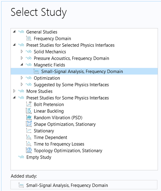
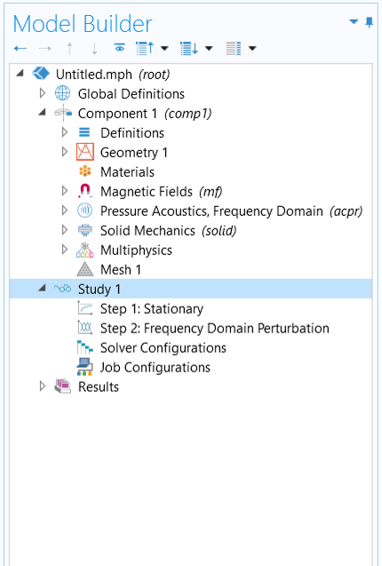
Selecting theSmall-Signal Analysis, Frequency Domainstudy from theSelect Studywindow (left) and the resulting study steps added to the model tree (right).

In Part 2 of this course, we will learn how to run a frequency-domain analysis. Then, in Part 4, we will look at setting up a transient model.

Solving the Problem in 2D or 3D

For structures with axial symmetry, a 2D axisymmetric model often suffices, assuming that the load conditions, boundary conditions, and the solution of interest exhibit the same symmetry. This applies to conventional dynamic drivers characterized by rotational symmetry (for instance, models that do not have a basket). Such models are especially useful when the aim is to capture the axisymmetric modes excited in both solid and fluid components. Implementing a 2D model considerably reduces the computational load, whereas you can easily visualize the results in a full 3D geometry using aRevolution 2Ddataset.

When a 2D axisymmetric model is not suitable, and a 3D model is required, check if your geometry has any symmetry (or near symmetry) and decide whether you anticipate that the solution will have similar symmetry. Taking advantage of symmetry enables you to model just a portion of the geometry, significantly reducing the complexity of a 3D model. The images below illustrate various geometry scenarios: 2D axisymmetry applied when the 3D geometry is entirely axisymmetric (left image); 3D modeling of a quarter of the geometry when a basket is incorporated, leveraging symmetries (middle); and a 3D model using a 60-degree sector when using sector symmetries (right). In these examples, the speaker driver is assumed to be placed in an infinite baffle.

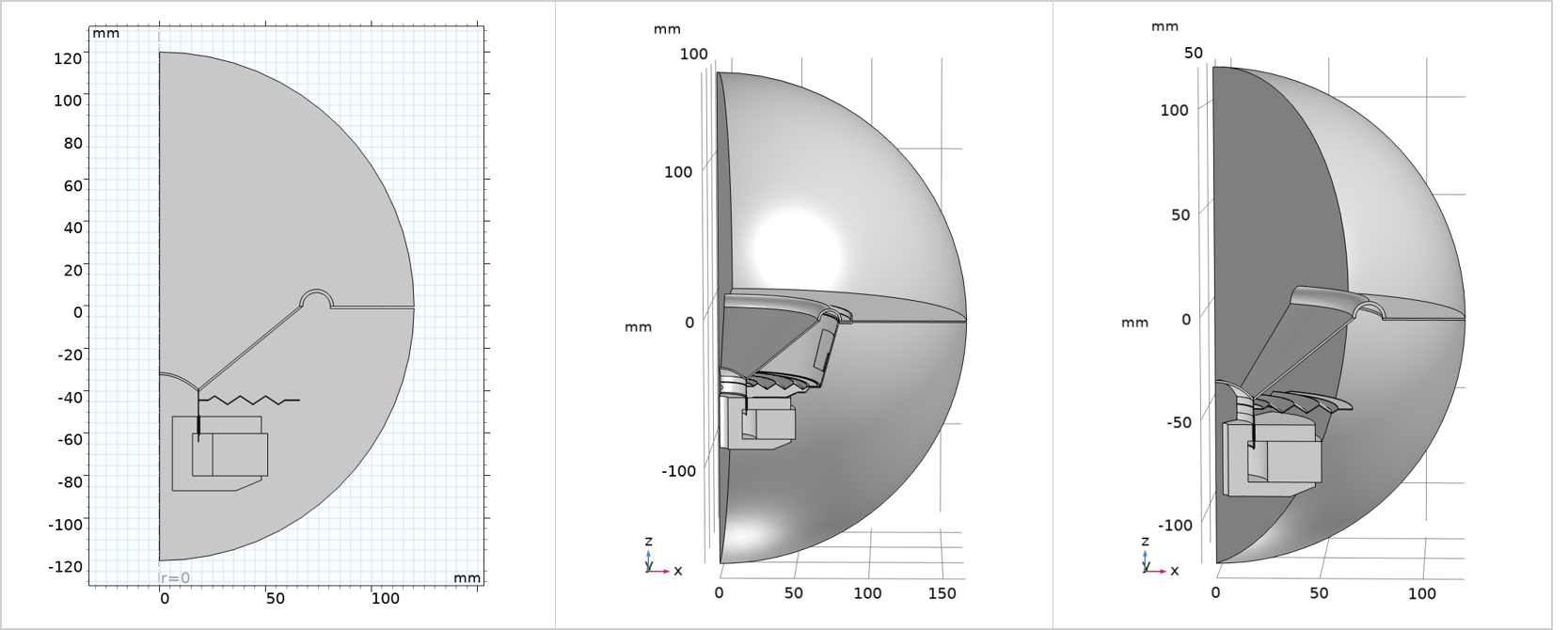Geometries for solving the problem in 2D axisymmetry (left), 3D with a quarter of the geometry by using symmetries (middle), and 3D with a 60-degree sector by using sector symmetries (right).

Extracting 2D Geometry From a 3D CAD

If you are working with a 3D CAD file and want to solve the model within a 2D axisymmetric space dimension, you can extract a cross section from the 3D model for 2D analysis. The following steps and images outline how to achieve this:

1. In a 3D component, import the 3D CAD geometry.
2. Use aWork Planefeature and set the plane to align with the cross section of the driver.

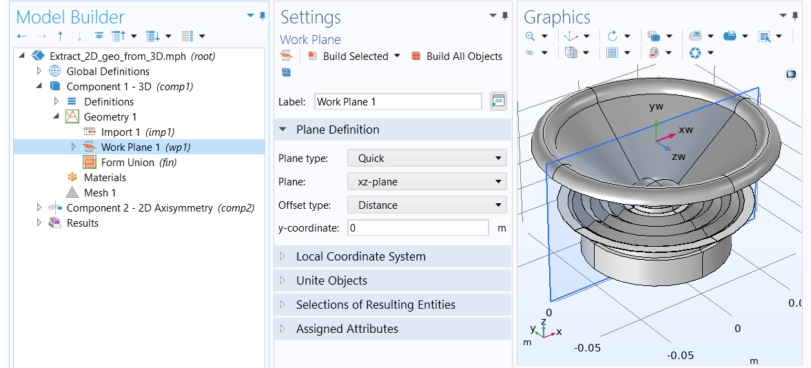The Model Builder with the Work Plane feature selected, the corresponding Settings window, and the driver model in the Graphics window. A work plane is defined to specify a cross section of the 3D object.

3. Add a 2D axisymmetric component (Component 2 - 2D Axisymmetry) to the model.
4. Use aCross Sectionfeature and select the work plane defined inGeometry 1ofComponent 1 - 3Dfor the cross section from theWork Planelist.

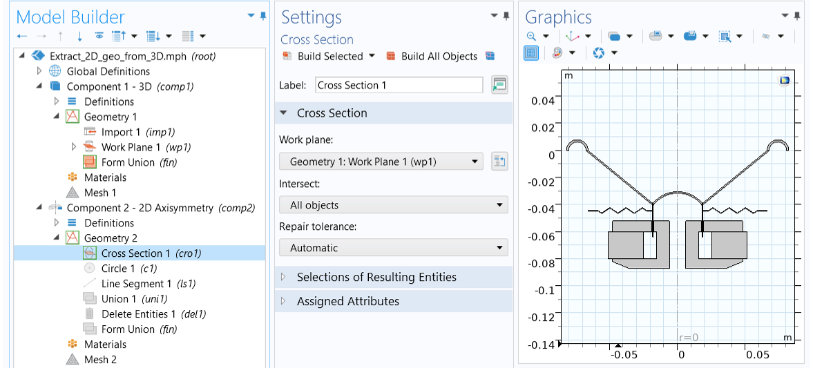The COMSOL Multiphysics UI showing the Model Builder with the Cross Section feature selected, the corresponding Settings window, and the Graphics window showing the 2D cross section. TheCross Section feature is used to create a 2D cross section from an intersection between a 3D geometry and a work plane.

5. You can then add fluid domains to the 2D geometry for multiphysics analysis.

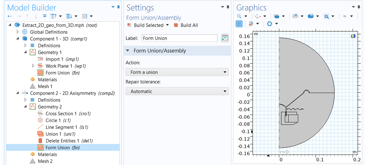The COMSOL Multiphysics UI showing the Model Builder with the Form Union setting selected, the Form Union/Assembly settings window, and the Graphics window with the 2D geometry. The final geometry for the 2D analysis.

The steps are demonstrated in the attached Extract_2D_geo_from_3D.mph file.

The Required Physics Interfaces and Multiphysics Couplings

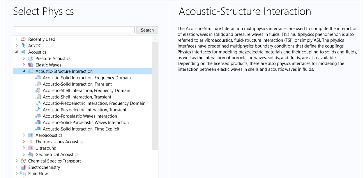
A full electrovibroacoustic analysis of the dynamic transducer requires using theMagnetic Fieldsinterface in the AC/DC Module to model the electromagnetic field. It also requires using one of theAcoustic-Structure Interactionmultiphysics interfaces in the Acoustics Module to model vibrations of the moving parts and the sound radiating into the surrounding air.

The Magnetic Fields Interface

TheMagnetic Fieldsinterface, found under theAC/DC>Electromagnetic Fieldsbranch in theSelect Physicspage of the Model Wizard, is used to compute the magnetic field and induced current distributions in and around coils, conductors, and magnets.

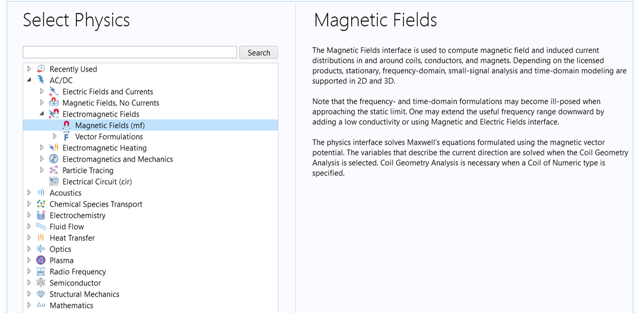TheMagnetic Fieldsinterface in theSelect Physicswindow.

The physics interface solves Maxwell’s equations and is used to compute, for example, the electric,, and magnetic,, fields.

TheMagnetic Fieldsinterface requires the following material properties:

• The electrical conductivity,
• The relative magnetic permeability,, or the magnetization vector,
• The relative permittivity,
• The velocity of the moving coil,
• The remanent flux density of the magnet,
• The B-H curve of the top plate and pole piece
• The coil properties, including the number of turns, the coil wire conductivity, and its cross-section area
• The externally generated current density,
• The frequency,(for a time-harmonic analysis)

The Acoustic–Structure Interaction Multiphysics Interfaces

There are multiple multiphysics interfaces in theAcoustic-Structure Interactionbranch that can be used to model coupled vibrations and sound radiation. The interfaces used most often are theAcoustic-Solid Interaction, Frequency Domaininterface for frequency-domain analysis and theAcoustic-Solid Interaction, Transientinterface for performing a time-dependent study. The following image shows the location of these interfaces in theSelect Physicswindow of the Model Wizard.

TheAcoustic-Solid Interactionmultiphysics interfaces are under theAcoustics > Acoustic-Structure Interactionbranch of theSelect Physicspage in the Model Wizard.

TheAcoustic-Solid Interactionmultiphysics interfaces combine thePressure AcousticsandSolid Mechanicsinterfaces to connect the acoustic pressure variations in a fluid domain with the structural deformation in a solid domain. When selecting this type of multiphysics interface, theAcoustic-Structure Boundarymultiphysics coupling feature is automatically added to the model. This multiphysics coupling is used to connect aPressure Acousticsmodel to any structural component.

You also have the option to add the acoustics and structural physics one at a time and then combine them by manually adding theAcoustic-Structure Boundarycoupling, which is readily available in the multiphysics selection list that appears after right-clicking theMultiphysicsnode in the model tree.

ThePressure Acousticsinterface solves a scalar wave equation for the total acoustic pressure,, while theSolid Mechanicsinterface solves Newton’s second law of motion for the structural displacement field,.

ThePressure Acousticsinterface requires the following material properties:

• The density,
• The speed of sound,
• The monopole domain source,(provides an option to add a domain mass source when applicable; the default value is zero)
• The dipole domain source,(provides an option to add a domain force source when applicable; the default value is zero)
• The frequency,(for a time-harmonic analysis)
• Damping parameters when a lossy fluid model is used to include bulk damping

TheSolid Mechanicsinterface requires the following material properties:

The density,A pair of elastic moduli for isotropic materials, or for anisotropic materials, either an elasticity matrix or a compliance matrix The body force,The frequency,(for a time-harmonic analysis) Damping parameters when mechanical damping is included

TheAcoustic-Structure Boundarycoupling includes the fluid load on the structure and the structural acceleration as experienced by the fluid. The image below shows an example of anAcoustic-Structure Boundarycoupling used in aloudspeaker driver simulation.

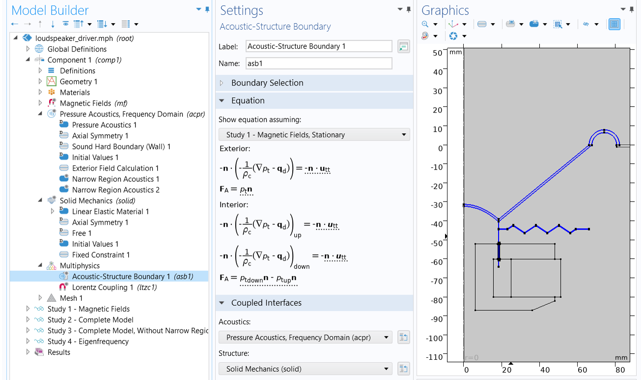The COMSOL Multiphysics UI showing the Model Builder with the Acoustic-Structure Boundary feature selected, the corresponding Settings window with a coupling between the Pressure Acoustics, Frequency Domain interface and Solid Mechanics interface set up, and the corresponding 2D model in the Graphics window. TheAcoustic-Structure Boundary multiphysics coupling connects a pressure acoustics model to any structural component.

The Lorentz Coupling

To calculate the Lorentz force and back EMF, use aLorentz Couplingfeature, which is a multiphysics coupling between theMagnetic Fieldsinterface and theSolid Mechanicsinterface.

When modeling dynamic drivers, the coupling is typically added in the voice coil domains, as seen in the image below. It passes the Lorentz force from theMagnetic Fieldsinterface to theSolid Mechanicsinterface and passes the structural velocity — which leads to the induced electric field — from theSolid Mechanicsinterface to theMagnetic Fieldsinterface.

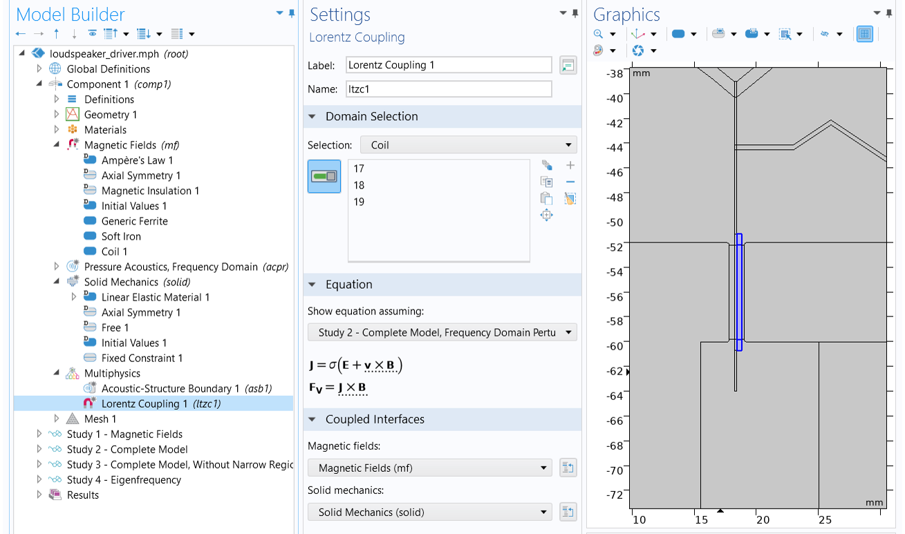The COMSOL Multiphysics UI showing the Model Builder with the Lorentz Coupling feature selected, the corresponding Settings window, and the Graphics window showing a close-up of the 2D model. TheLorentz Coupling connects the magnetic fields with solid mechanics to calculate the Lorentz force and back EMF.

Other Physics Interface Options for Structural Vibrations and Acoustics

Modeling Thin Structures Using the Shell Feature

When there are thin objects in the system subject to vibrations, using theShellfeature can vastly reduce the number of mesh elements required to resolve the model. TheShellinterface is available for 3D and 2D axisymmetric analysis. You can consider using it for thin components, including the cone, the surround, the spider, and the former, as well as thin mounting panels like cabinet walls if applicable. However, the coil object needs to be modeled as a solid domain using aSolid Mechanicsinterface since theLorentz Couplingfeature is only applicable for coupling theMagnetic Fieldsinterface with theSolid Mechanicsinterface.

TheAcoustic-Structure Boundarycoupling is also applicable for coupling aPressure Acousticsmodel with aShellmodel. When the shells are interior structures with fluid on both sides, a slit is added to the pressure variable and care is taken to couple the ’up’ and ‘down’ sides such that the acoustic load is given by the pressure drop across the thin structure.

Solid–Thin Structure Connection

When both theShellandSolid Mechanicsinterfaces are used, theSolid-Thin Structure Connectionmultiphysics coupling feature can be added to create transitions between domains modeled using theSolid Mechanicsinterface and boundaries modeled using theShellinterface. See an example in theLoudspeaker Driver in a Vented Enclosuretutorial model.

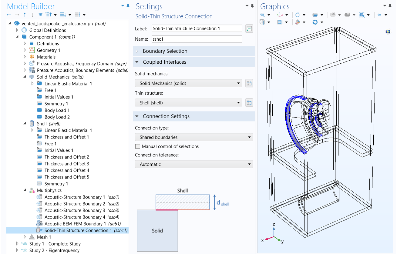The COMSOL Multiphysics UI showing the Model Builder with the Solid-Thin Structure Connection feature selected, the corresponding Settings window, and the model in the Graphics window. TheSolid-Thin Structure Connection couples shells and solids.

TheShellandSolid-Thin Structure Connectionfeatures require the Structural Mechanics Module.

Modeling Thermoviscous Boundary Layer Losses

When sound propagates in structures and geometries with small dimensions, the sound waves become attenuated because the losses occur in the acoustic thermal and viscous boundary layers near the walls. Including these losses are important. In order to accurately model the response of small transducers, like miniature loudspeakers (especially when operated around resonant frequencies), it is important to include these losses.

COMSOL^®provides three ways to model thermoviscous boundary layer losses:

Use theNarrow Region Acousticsfeature with thePressure Acoustics, Frequency Domaininterface. This defines a fluid model in channels and ducts of constant cross section. The losses due to the viscous and thermal dissipation in the acoustic boundary layer are homogenized and smeared on the fluid. Although applicable only in waveguides of constant cross section, it is suitable for all frequencies, that is, also the very narrow case where boundary layers are overlapping. Examples of this option include theLoudspeaker Driver - Frequency Domain Analysis,Balanced Armature Transducer - Frequency Domain Analysis, andOW Microspeaker: Simulation and Correlation with Measurementstutorials.

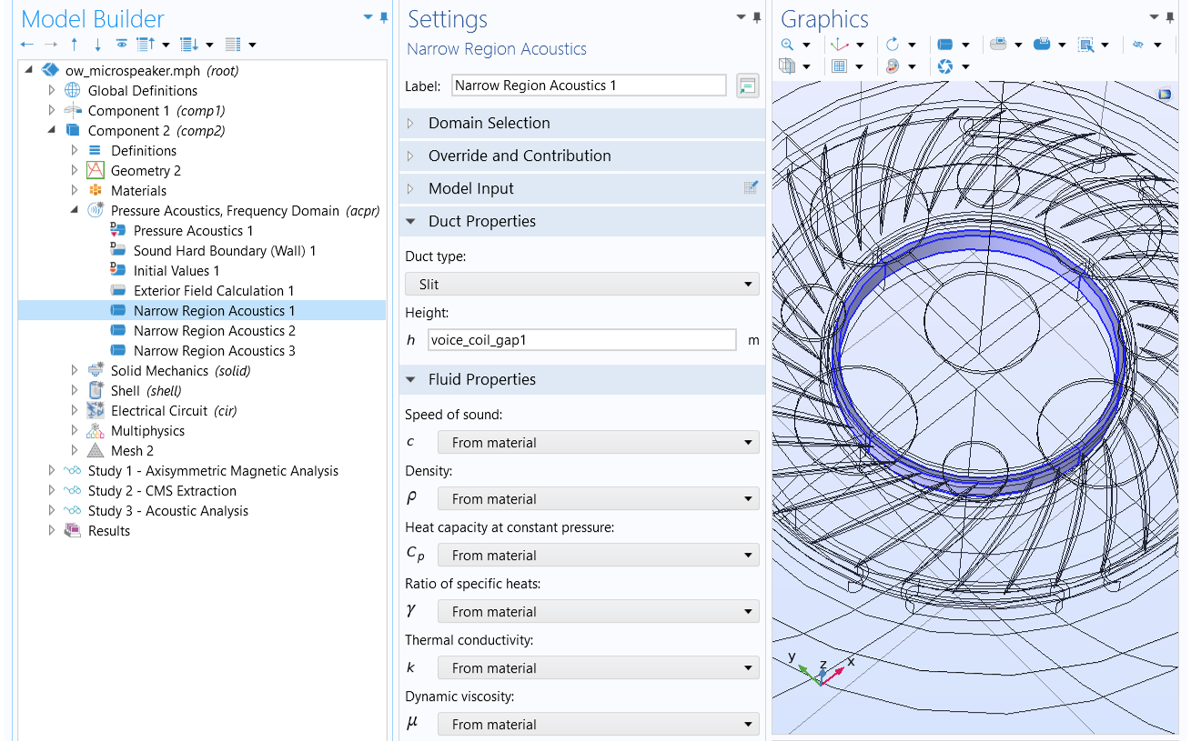An example of usingNarrow Region Acousticsto capture the thermoviscous damping in small fluid channels of constant cross section.

Use theThermoviscous Boundary Layer Impedancefeature with thePressure Acoustics, Frequency Domaininterface. With this feature, the losses are integrated through the boundary layers in an analytical manner. This feature is not suitable for geometry with overlapping boundary layers, such as geometry with very curved boundaries or very narrow waveguides (where the dimensions are comparable to the boundary layer thickness). Other than these cases, there are no restrictions for when this feature can be used with a certain geometry shape. See a demonstration of this feature in theEar Canal AcousticsandType 4.3 Ear Simulatortutorials.

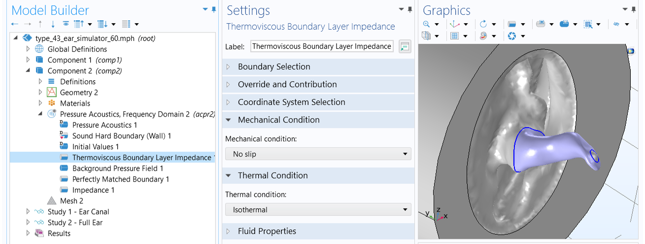An example of using theThermoviscous Boundary Layer Impedancefeature to capture the thermoviscous damping in small fluid channels where boundary layers are not overlapping.

Use a thermoviscous acoustics physics interface that models the acoustic behavior in the thermoviscous boundary layer in detail. It solves a full set of linearized governing equations including explicitly thermal conduction effects and viscous losses. Not limited to any geometry and dimension, this option works for the full frequency range and supports both the frequency domain and transient analysis. Examples include thePiezoelectric MEMS Speakerand theElectrostatic Speaker Drivertutorial models.

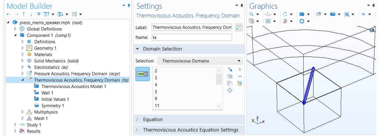The full thermoviscous acoustic model is used to simulate the acoustic behavior in the narrow gaps of air between the triangular membranes of a piezoelectric MEMS speaker.

In addition, note that in order to solve a thermoviscous acoustic model, you must solve for the acoustic pressure; the velocity field (has 3 components in a 3D model); and temperature variations. With this many dependent variables, your acoustics model may be computationally expensive and require many degrees of freedom (DOFs). It is therefore recommended that you first check if you are able to use the first two effective options before turning to the full thermoviscous formulation.

Thermoviscous Acoustic–Structure Boundary

TheThermoviscous Acoustic-Structure Boundaryfeature is used to couple aThermoviscous Acousticsinterface with any structural component. The coupling prescribes continuity in the displacement field at the fluid–structure boundaries.

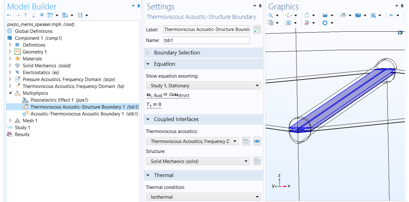TheThermoviscous Acoustic-Structure Boundarycoupling prescribes continuity in the displacement field at the fluid–structure boundaries.

Acoustic–Thermoviscous Acoustic Boundary

As it is only necessary to solve the fully-detailed thermoviscous acoustics model near walls in the boundary layer region, it makes sense to switch to classical pressure acoustics outside this region. This approach saves a lot of memory and solution time due to the reduced number of degrees of freedom. In this case, you can use theAcoustic-Thermoviscous Acoustic Boundarycoupling feature to couple aThermoviscous Acousticsinterface with aPressure Acousticsinterface.

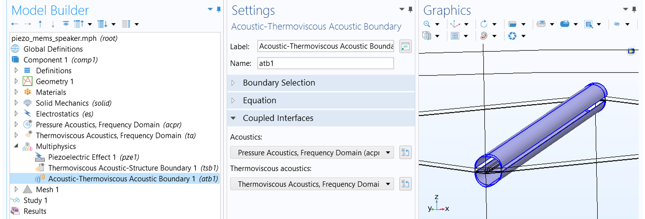TheAcoustic-Thermoviscous Acoustic Boundarycoupling connects a thermoviscous acoustics model with a pressure acoustics model.

The coupling prescribes continuity in the total normal stress (dynamic condition) and the total normal acceleration for the mechanical part (kinematic condition). An adiabatic condition is prescribed for the total temperature to match the physical assumptions of the pressure acoustics formulation.

Further Learning

Read the following blog posts to learn more about thermoviscous acoustics and the multiphysics coupling features in COMSOL Multiphysics^®for modeling different types of speaker drivers:

• Theory of Thermoviscous Acoustics: Thermal and Viscous Losses
• How to Model Thermoviscous Acoustics in COMSOL Multiphysics
• Modeling Speaker Drivers: Which Coupling Feature to Use

Also seeSupplement A - Equationsfor additional information.