学习中心

Defining Multiphysics Models Manually with User-Defined Couplings

---

In COMSOL Multiphysics^®, you can manually administer couplings between physics interfaces for which no coupling features are available. We refer to this as the manual approach with user-defined couplings. Here, we discuss how to implement the approach with a combination of physics phenomena in your model. The approach requires more effort to implement than themanual with predefined couplings approachand completely contrasts theautomatic approach, which provides an almost fully automated implementation.

When to Use the Manual Approach with User-Defined Couplings

When there is no alternative predefined option to define the multiphysics couplings in a model, there is functionality in the software that provides you with the flexibility to manually implement custom multiphysics couplings. This is done through user-defined variables, expressions, equations, or functions to couple different physics interfaces. We refer to this multiphysics modeling approach as the manual with user-defined couplings approach, since it involves manually administering the coupling and interaction between physics interfaces.

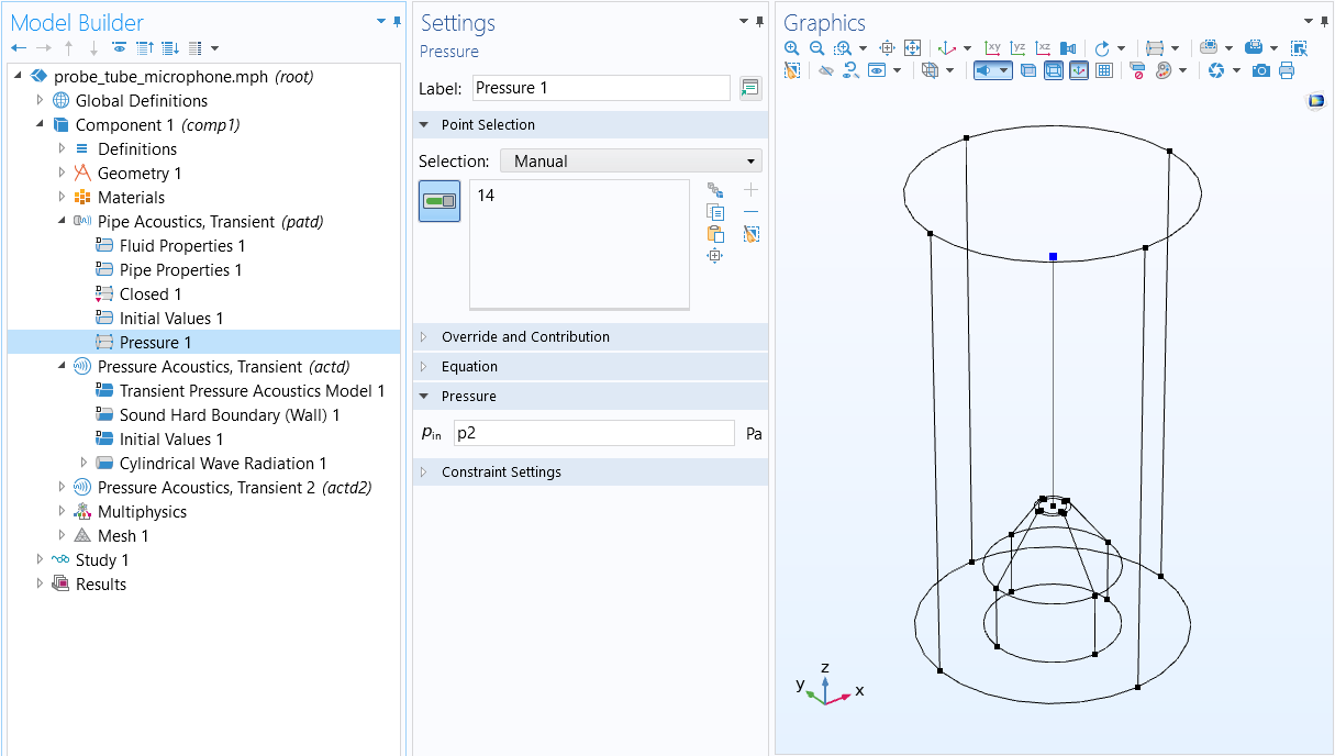The Model Builder in COMSOL Multiphysics, with the model tree showing the Pressure condition selected, the Settings window showing the Pressure condition settings, and the Graphics window showing the model geometry.
ThePressure condition in theprobe tube microphonetutorial model, which is used for manually coupling the 1D (pipe) and 3D (exterior) domains in the model.

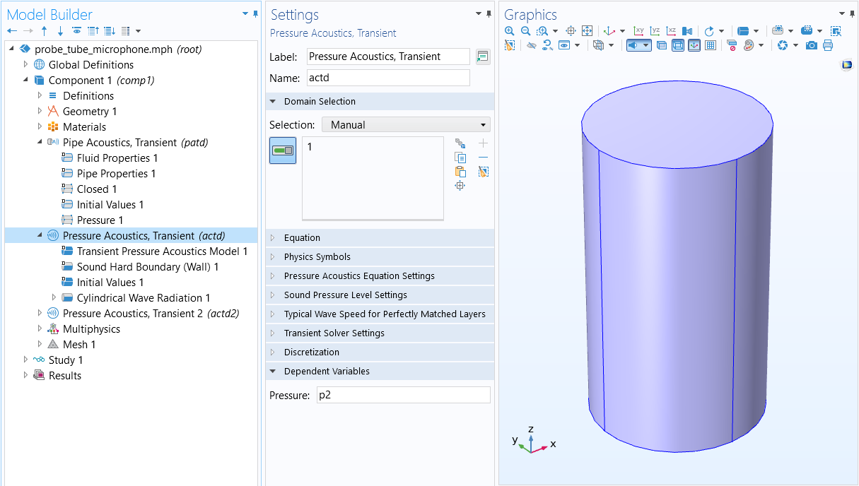The Model Builder in COMSOL Multiphysics, with the model tree showing the Pressure Acoustics, Transient condition selected, the Settings window showing the Pressure Acoustics, Transient condition settings, and the Graphics window showing the model geometry.
ThePressure Acoustics, Transient interface of theprobe tube microphonetutorial model, wherein the dependent variable,p2 , is used to manually couple it to thePipe Acoustics, Transient interface through aPressure condition (as pictured in the previous screenshot).

This approach is wide and vast with respect to how it can be implemented for defining multiphysics models. There is no standard that dictates how it necessarily should or can be implemented, as it will vary depending on what is being modeled. Some examples include using expressions to make material properties or boundary conditions functions of the dependent variables of another physics interface.

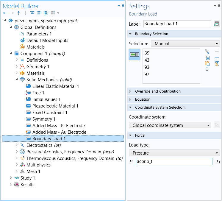
In thePiezoelectric MEMS Speakertutorial model, aBoundary Loadis used to manually couple theSolid Mechanicsinterface andPressure Acoustics, Frequency Domaininterface. However, this is also available as a predefined multiphysics coupling in the Acoustics Module.

A screenshot of the model tree with the Equation View option under the Pressure Acoustics node selected, with the list of variables shown on the right.
Equation View for thePressure Acoustics node, from which a variable is used for a boundary condition in another physics interface (as pictured in the previous screenshot) in order to manually couple the two physics interfaces.

Since this approach requires that you know the equation formulation in detail, and since you have to enter equation contributions manually, it is the most error-prone and usually also the most laborious way of defining multiphysics models. This is why we recommend utilizing thefully automatic approachormanual approach with predefined couplingswhenever possible. However, even the manual approach is straightforward to use and gives you full control of the model definition. Although there are readily available predefined multiphysics interfaces and couplings, user-defined couplings are often used in teaching to show students how different equations describing different physics phenomena can be coupled manually. The upside is that you have the predefined multiphysics couplings as reference to compare with. But in most cases, the manual, user-defined couplings are used when there is no predefined multiphysics coupling available. Some guidelines and suggestions on how a manual multiphysics coupling can be implemented are discussed below.

Procedure to Implement the Approach

As noted earlier, the manual approach using user-defined couplings can be implemented in a variety of different ways. Although there is no explicit sequence of steps that must be followed, the general procedure for using the approach is as follows:

1. Add the physics interfaces
2. Define the physics settings (material properties, boundary conditions, initial conditions, etc.)
3. Repeat steps 1 and 2 for each subsequent physics interface
4. Define the multiphysics couplings

As noted earlier, since this approach is the most prone to errors, it is important to always check your results after computing the model. You'll notice that defining the physics settings is split into two parts: defining each individual physics interface and then defining the multiphysics couplings. Each physics interface defines its dependent variables and a set of derived variables. A dependent variable may be, for example, the temperature variable. Derived variables may be the components of the heat flux vector, which are defined using the temperature variable. The heat transfer equations are solved for the temperature, while the heat flux components may be used to formulate these equations or to generate streamline and arrow plots when the temperature field is obtained in the solution.

You can define multiphysics couplings by creating your own derived variables of the dependent variables. You can also directly type in expressions of dependent variables in any physics setting's edit fields. However, creating your own variables is a good way of administrating multiphysics couplings. For example, you can create a derived variable for the heat source in a heat transfer model that depends on the electric field. You can do this in theDefinitionsnode by adding aVariable. You can then enter the heat source derived variable in the heat source edit field in the heat transfer settings. A derived variable can be an arbitrary expression of any dependent variable and its derivatives. Once a variable is defined, you can use it to describe sources, material properties, fluxes, forces, boundary conditions, initial conditions, or any other input in the physics interfaces. You can simply type in expressions containing dependent variables, derivatives of dependent variables, and derived variables in the input edit fields for any of the the physics settings in the UI.

The derived variables defined and used internally by COMSOL Multiphysics^®can be inspected and changed directly in the UI. By clickingShow More Optionsin theModel Buildertoolbar and selecting theEquation Viewcheck box in the dialog box, all variables and equation contributions defined by each node in a physics interface become visible and editable.

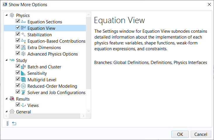
Enable showing theEquation Viewnodes in the model tree by clicking the respective check box.

This means that you can directly change or add terms to the already predefined derived variables. For example, assume that you want to add a contribution to an already defined heat source. Then you can locate the corresponding derived variable in theEquation Viewnode settings and add the contribution, which may, for example, be an expression of the electric potential. In the edit fields inEquation View, you can enter any expression of a dependent variable, derivatives of dependent variables, and other derived variables.

Below, we show how you can used derived variables and theEquation Viewnode settings to define multiphysics couplings.

Walkthrough Example: Modeling Resistive Heating and Thermal Expansion

Similar to the other articles discussing the other approaches for defining multiphysics models, let's use thethermal microactuator tutorial modelto show how we would define the multiphysics effects manually. Also, similarly to the other articles, it is assumed that all details regarding the model setup, except for the physics, have been completed. A detailed overview of the device and the physics involved in its operation are described in the Learning Center article introducing the fully automatic approach.

Note: For this combination of physics phenomena, a predefined multiphysics interface, theJoule Heating and Thermal Expansionmultiphysics interface, is available to be used and is what we would add to our model instead of using this approach. We recommend employing either the fully automatic or manual with predefined couplings approach for defining the multiphysics in your models whenever possible, as the manual with user-defined couplings approach requires a completely manual implementation. The following walkthrough is meant for demonstration purposes only.

Following the procedure we listed above for implementing this approach would result in us first adding and then defining the physics settings for the electrical part of the model, then the thermal part of the model, and finally the structural part of the model. Thus, the physics settings have been defined, omitting all multiphysics effects, for each of the subsequent physics interfaces:Electric Currents,Heat Transfer in Solids, andSolid Mechanics, respectively. Please note that the physics settings can be defined in any order.

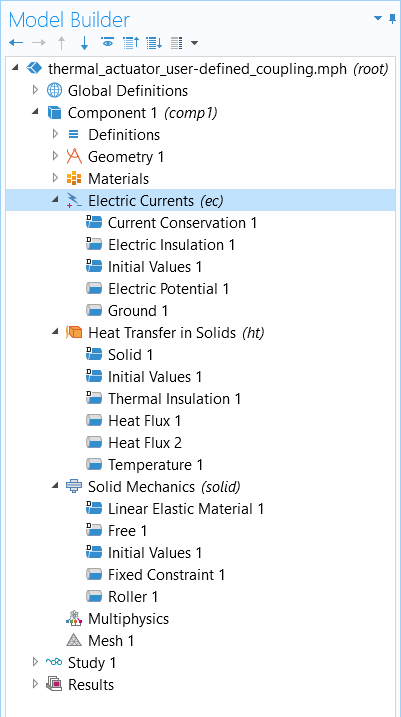
The model tree thus far for the thermal microactuator tutorial model, with the multiphysics effects not yet accounted for.

After defining the settings for each physics interface, we need to determine how we should define the couplings between the physics interfaces. Think about how the physics phenomena are interacting. Does one physics phenomena serve as causation of, or contribute to, another physics phenomena? We should allow the multiphysics phenomena occurring itself to naturally dictatewhereandhowwe define the multiphysics effect in a model.

Joule Heating

Since the electric heating is a heat source, it would be logical to define the effect under theHeat Transfer in Solidsinterface and use an expression that is a function of the electric field and the electric conductivity. We also know that the heat source may be present everywhere in the model domain in this case. We can therefore select thePhysicsribbon tab, while theHeat Transfer in Solidsinterface is selected, and locate theHeat Sourcefeature under theDomainsmenu to create the multiphysics coupling.

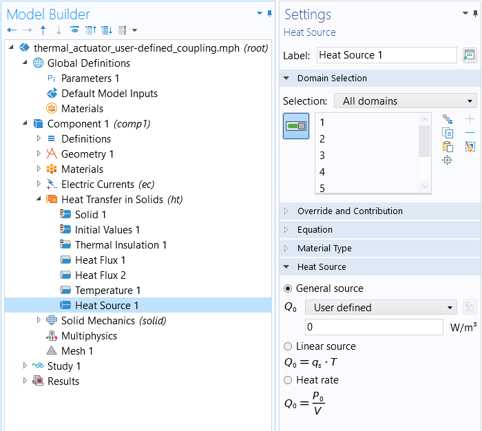
TheHeat Sourcenode.

We want to locate the electric losses and add them as a heat source in the heat transfer equations (temperature equations). So now we need to use an expression that describes this quantity. We could define it manually, since we know that the electric heating is the scalar product of the current density vector and the electric field,. However, in this case, this is already predefined in COMSOL Multiphysics^®. We can locate the electric heating term under theCurrent Conservationnode and enable displaying theEquation Viewnode to access all the variables and expressions used by that physics node. There, we'll find the variableec.Qrh, which describes the electric heating in the domain. We can see how this derived variable is defined. As we expected, it is formed by the scalar product of the current density vectorand the electric field vector, which are also defined as derived variables. The dependent variable here is the electric potential, V, and the derived variables for the current density vector and the electric field use this variable in their definition (actually the gradient of the electric potential). In the same way as COMSOL Multiphysics^®internally defines its derived variables, we can also use this syntax to create our own derived variables, if needed. We can also edit the derived variables defined by COMSOL Multiphysics^®in their corresponding edit field. In this case, we have the benefit of the electric heating term already being defined as a derived variable. We can use this variable as the expression for the value in theHeat Sourcedomain node.

All these steps can be avoided, since the electric heating is predefined and can be added automatically by the multiphysics node. However, in cases when a coupling is not predefined, you would use the strategy outlined above.

A screenshot of the Model Builder, with the model tree on the left showing the Equation View node selected under the Current Conservation node, with the Settings window on the right.
TheEquation View node for theCurrent Conservation node. The variableec.Qrh is used to introduce electric heating as a heat source in the modeling domain, i.e., to couple the equations for the electric potential with the equation for temperature.

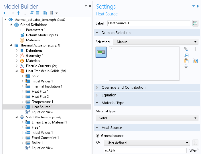
TheHeat Sourcedomain feature with the updated settings for the value applied.

Thermal Expansion

Next, we need to define the thermal expansion that couples theSolid MechanicsandHeat Transfer in Solidsinterfaces. Since thermal expansion gives a contribution to the strain tensor, we need to locate the strain tensor in theSolid Mechanicsinterface and add the expression for thermal strain. In this case, we need the strain tensor formulation in one of theEquation Viewsubnodes to theStructural Mechanicsinterface. We can search for the strain tensor by using theFind toolby pressingCtrl-Fand enteringstrain tensorin the search dialog box. TheFind Resultstable is then updated in the window below theGraphicswindow. Double-clicking on one of the strain tensor components listed in theFind Resultstable takes us to the correctEquation Viewnode. For the device we are modeling, the relevantEquation Viewis the subnode to theLinear Elastic Materialnode. We can add the thermal strain contribution as an expression of temperature,T, in the respective strain tensor component.

Note: You can also couple the physics for this model by addingThermal Expansionas a subnode to theLinear Elastic Materialnode. However, we will ignore that such a feature is available for the purposes of this demonstration to implement the manual approach using user-defined couplings.

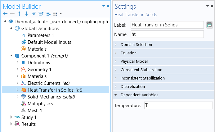
The dependent variable,T,for theHeat Transfer in Solidsinterface, which we can incorporate into expressions used for theSolid Mechanicsinterface.

Enabling theEquation Viewallows us to access all the variables and the expressions used for theLinear Elastic Materialnode. Here, we can modify the equations to define any coupling between the strain and temperature.

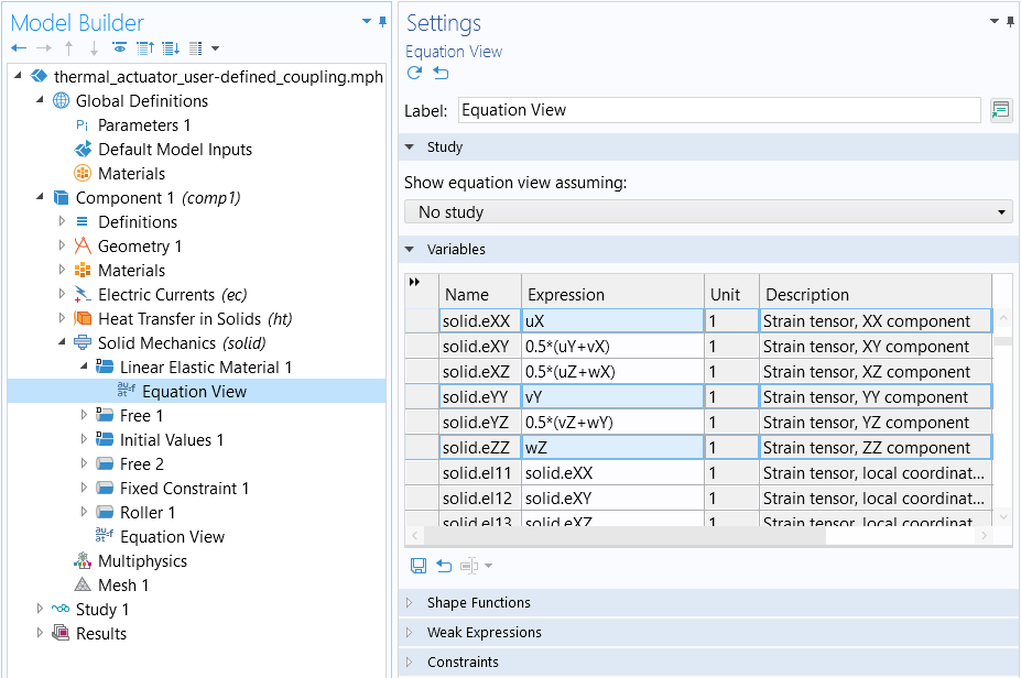A screenshot of the Equation View subnode to the Linear Elastic Material node selected in the model tree, with the Settings window open on the right.
TheEquation View subnodeSettings window, wherein the variables and the respective expressions that will be modified are selected in the table and highlighted in blue.

We'll want to modify the strain definition for the variablessolid.eXX,solid.eYY, andsolid.eZZusing the equation for thermal strain,

whereinαis the material's thermal expansion coefficient,Tthe temperature field, andT₀is the strain reference temperature. The values forαandT₀are known and defined by the parametersalphapsandT0, respectively. We can add the contribution to the strain tensor components as seen in the screenshot below. Note that this expression for thermal expansion is valid only for relatively small deformations, which we may assume that we have in our case.

A screenshot of the Settings window for the Equation View subnode, with warning icons shown for different variables in the list.
TheEquation View subnode for theLinear Elastic Material node. The expressions for the variables highlighted with a warning icon have been edited to account for thermal strain.

To see this approach be implemented for modeling this combination of physics, you can watch the video below for a full demonstration.

Tutorial: Defining a Multiphysics Model Using the Manual Approach with User-Defined Couplings

Modeling Exercises

Demonstrate the knowledge you have gained from this article by putting it into practice with the follow-up modeling exercises listed below. The directions provided for each modeling exercise contain all the information necessary in order to complete it, but are intentionally generalized to encourage self-guided problem-solving. You can check your implementation with the solution model files provided by comparing them manually or using theComparison toolto exactly identify the differences.

1. Previously, you built the busbar tutorial model using the fully automatic approach and the manual approach with predefined couplings. Now, use the manual approach with user-defined couplings to define the physics for this model. Follow thedirectionsprovided to define the physics setup. The geometry is available to download:busbar.mphbin.
2. Previously, you built the free convection tutorial model using the fully automatic approach and the manual approach with predefined couplings. Now, use the manual approach with user-defined couplings to define the physics for this model. Follow thedirectionsto define the physics setup. The geometry is available to download:free_convection.mphbin.
3. Previously, you built the convective cooling of a busbar tutorial model using the manual approach with predefined couplings. Now, follow thedirectionsprovided to define the physics for the model using the manual approach with user-defined couplings. The geometry is available to download:busbar_box.mphbin.