学习中心

Finite Element Frequency-Domain Analysis in 3D

---

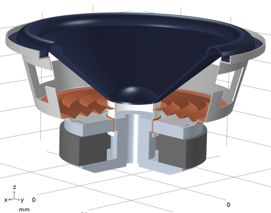
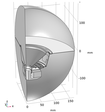
When any of the assumptions required for a 2D axisymmetric model is not valid, you need to solve the problem in 3D. Here, we use the geometry shown below as an example to discuss the extra considerations for modeling a dynamic speaker driver in 3D. The model is based on a 3D representation of the 2D axisymmetric analysis we conducted in Part 2 of this course. The geometry is modified to include a basket and other details, which are not axisymmetric anymore but possess symmetry in the x = 0 and y = 0 planes. We briefly mentioned in Part 1 that exploiting symmetry can reduce the size of a 3D model effectively. Here, a quarter of the geometry (as seen below on the right) is used with symmetry conditions applied in the physics. This setup captures all the 3D modes that possess these symmetries.

The structure of the speaker driver (left) and the geometry used in the analysis (right) for a quarter of the driver, where symmetry conditions are used.

Coil Geometry Analysis

TheCoilfeature requires additional settings in 3D models to determine the geometry and the direction of the current flow. When theHomogenized multiturnfeature is used, theCoil typeinput determines how the direction of the current flow is specified. The available alternatives areLinear,Circular,Numeric, andUser defined. The most often usedNumericoption computes the current flow in a dedicated preprocessing study step,Coil Geometry Analysis, as shown in the image below. The other three options do not require any preprocessing. Note that theCoil Geometry Analysisstudy step must precede the main study steps and that it only solves for theMagnetic Fieldsphysics interface.

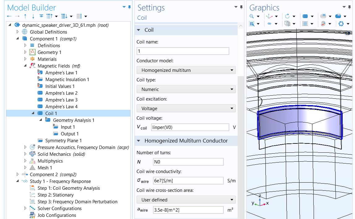The COMSOL Multiphysics UI showing the Model Builder with the Coil feature selected, the corresponding Settings window, and the dynamic speaker model in the Graphics window.

TheCoilfeature requires additional settings in 3D models to determine the geometry and the direction of the current flow.

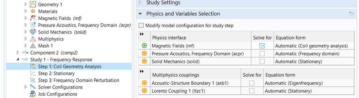A close-up of the Coil Geometry Analysis feature selected in the Model Builder and the tables in the Physics and Variables Selection section of the Settings window.

A coilGeometry Analysisstudy step is necessary for aNumericcoil type.

The computation of the current flow in the coil requires additional information on the coil geometry, which you can provide in the defaultGeometry Analysissubnode and theInput/Outputboundary conditions under it. If the model represents only a section of the geometry obtained from symmetry cuts (such as a quarter of the entire coil, as in this tutorial), use theSymmetry specificationsettings to add appropriate correction factors. Enter theCoil length multiplication factor F_LandCoil area multiplication factor F_A(dimensionless integer numbers). The actual length of the coil (used for computing the coil voltage and resistance) is computed as the productF_L·L, whereLis the domain length. The coil's cross-section area is computed asF_A·A, whereArepresents the cross-section area of the domain. During theCoil Geometry Analysisstudy step, the values ofLandAare automatically computed.

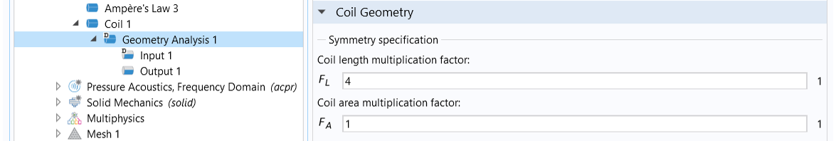A close-up of the Geometry Analysis subnode selected in the Model Builder and the Coil length multiplication factor and Coil area multiplication factor settings in the Settings window.

A correction factor of 4 is used to specify theCoil length multiplication factor F_Lwhen only a quarter of the coil length is modeled using symmetry conditions.

AnInputsubnode is added by default to theGeometry Analysisnode. Use it to specify the boundaries where the wires enter the domain or, in the case of a closed-loop coil, an interior boundary crossed by the wires. Used in combination with anOutputnode (forGeometry Analysis), it also defines the direction of the current flow in an open coil (fromInputtoOutput).

Applying Symmetry Conditions in the Physics

The geometrical symmetries need to be specified using symmetry boundary conditions when setting up the model. You can simply use the built-in symmetry features that are available for all the physics required for this analysis.

The Symmetry Feature

In pressure acoustics, this boundary condition sets the normal component of the acceleration (and thus the velocity) to zero:

For zero dipole domain source () and constant fluid density (), this means that the normal derivative of the pressure is zero at the boundary:

In thermoviscous acoustics, theSymmetrycondition corresponds to aSlipcondition (i.e., zero normal velocity, and therefore also zero tangential stress) for the mechanical degrees of freedom and theAdiabaticcondition (i.e., zero heat flux) for the temperature variation.

For structural mechanics, theSymmetrycondition sets the normal displacement to zero:

For magnetic fields, this feature is namedSymmetry Planeand it sets the normal magnetic flux density to zero:

Symmetry Setup for Exterior Field Calculation

The symmetry conditions used by the model also need to be reflected in theExterior Field Calculationsettings in order to get the correct exterior field, as seen in the image below.

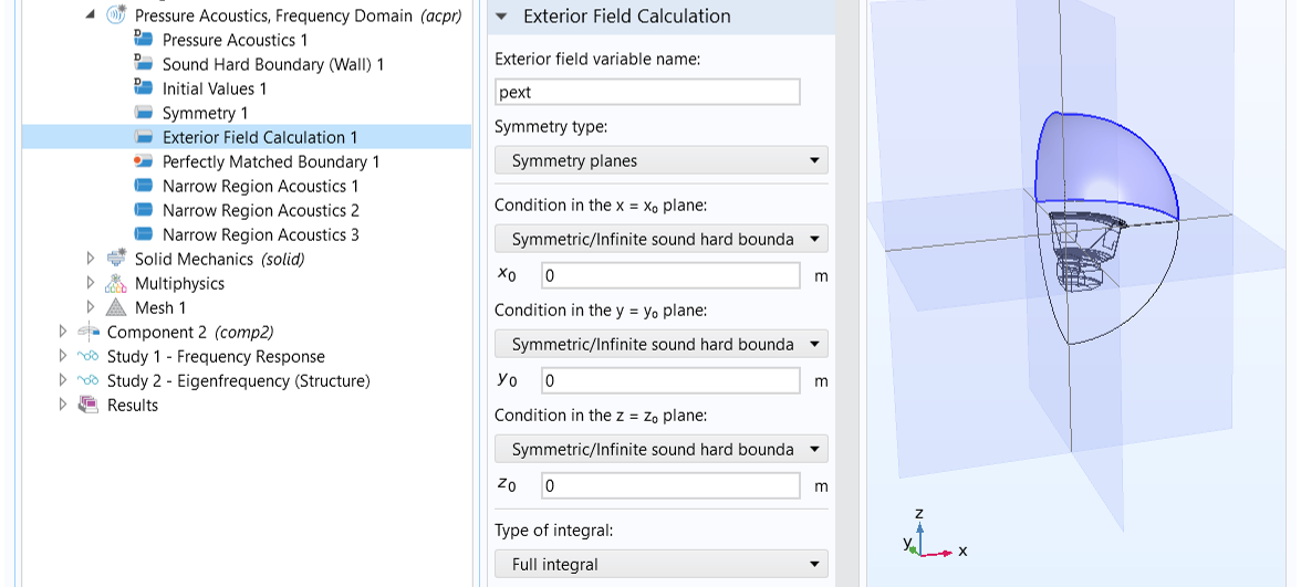A close-up of the Exterior Field Calculation feature selected in the Model Builder and the corresponding settings and model.

Symmetry conditions need to be reflected in theExterior Field Calculationsettings in order to get the correct exterior field.

Select theSymmetry typethat applies to the problem. The symmetry type and subsequent settings should match the conditions used in the underlying acoustics problem. AvailableSymmetry typeoptions includeSymmetry planes(the default),Sector symmetry, andSector symmetry with one symmetry plane.

TheSymmetry planesoption is applicable when all symmetry planes align with one of the Cartesian coordinate planes (with a possible offset), which is the case for this 90^°sector example and is thus used here. Note that an infinite baffle located at z = 0 is mathematically identical to a symmetry plane at z = 0, and this also needs to be included in the symmetry setup for exterior field calculation.

TheSector symmetryoption is used for a geometry representing only a sector (a subdivision of a full 360^°rotation). This allows you to obtain exterior field solutions when one of the symmetry planes is not aligned with any of the Cartesian coordinate planes, for example, when modeling a 60^°or 30^°sector.

TheSector symmetry with one symmetry planeoption allows for the combination of sector symmetry and a single symmetry plane. This is useful when you need not only theSector symmetryto reflect the geometry but also a symmetry plane to take into account an infinite baffle. See a demonstration of this option in the attached example,dynamic_speaker_driver_3D_sector_symmetry.mph, where a 60^°sector of a 3D speaker geometry is modeled.

Using Iterative Solvers for Large Models

As discussed earlier, a 3D speaker driver model usually requires solving for the coil geometry to get the coil property. Therefore, a complete study typically includes the following three study steps:

1. Use aCoil Geometry Analysisthat solves for theMagnetic Fieldsinterface only. This is necessary for computing the current flow of aCoilfeature in 3D models.
2. Use aStationarystudy that solves for theMagnetic Fieldsinterface only. This is used to calculate the static (DC) magnetic field generated by the permanent magnet.
3. Use aFrequency Domain Perturbationstudy that includes all the physics interfaces and all the multiphysics couplings. With this, we compute the frequency response (AC) about the biased solution.

For smaller problems, using a direct solver is often the best choice. Direct solvers have the advantage of being the most robust and general, however, they have the drawback of being memory hungry with increasing problem size. For larger problems, especially in 3D, the only option is often to use an iterative method. In comparison to direct solvers, iterative solvers require less memory and time (for large problems), and these scale more favorably with increasing model size.

However, iterative solvers may struggle with convergence when solving for magnetic fields, requiring special attention to enhance solver performance, as described in the next section.

Improving Iterative Solver Convergence for Low Frequencies

Iterative solvers may show slow convergence at low frequencies, which is discussed in part ofour Modeling Electromagnetic Coils course. The solution is to add a small artificial numerical electrical conductivity to all nonconducting materials that are included in the magnetic field analysis. To keep the induced current at a minimum value in these nonconducting domains, the artificial conductivity should be chosen so that the artificial skin depth is much larger than the size of the nonconducting volume. You can use the following formula to estimate an appropriate value for the numerical electrical conductivity,:

whereis the study frequency,is the permeability of vacuum, andis the artificial skin depth.

For this 3D dynamic speaker driver tutorial example, the nonconducting materials involved in the magnetic field analysis include the magnet, air, former, and spider. The size of the nonconducting region is around 165 mm, and it is recommended to use a frequency-dependent electrical conductivity so that the skin depth is much larger than 165 mm for all study frequencies. A process for manually implementing a small, artificial numerical electrical conductivity to these nonconductive domains is described below. Note that in versions 6.2 and up aFree Spacefeature is available, which completely automates this process for the air domains, the implementation of which can be seen in thetutorial model documentation

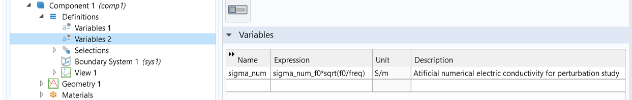
The images below demonstrate a way to estimate the suitable electrical conductivity for the entire frequency range. Firstly, a middle study frequency of 500 Hz is picked as the evaluating point (f0), and the numerical electrical conductivity required for this frequency, a parameter namedsigma_num_f0, is defined in the globalParametersnode (top image) to have a skin depth that is 20 times of 165 mm. This value is then used to define a frequency-dependent electrical conductivity variable (sigma_num) inComponent 1, using the expressionsigma_num_f0*sqrt(f0/freq), wherefreqis the internal variable for study frequency (bottom image). Note that the variablefreqis only available in the perturbationbf study step, and therefore this definition is applicable only (and necessary only) in that specific step. For the first two study steps,sigma_numis simply zero, which is defined in a separateVariablesnode (middle image).

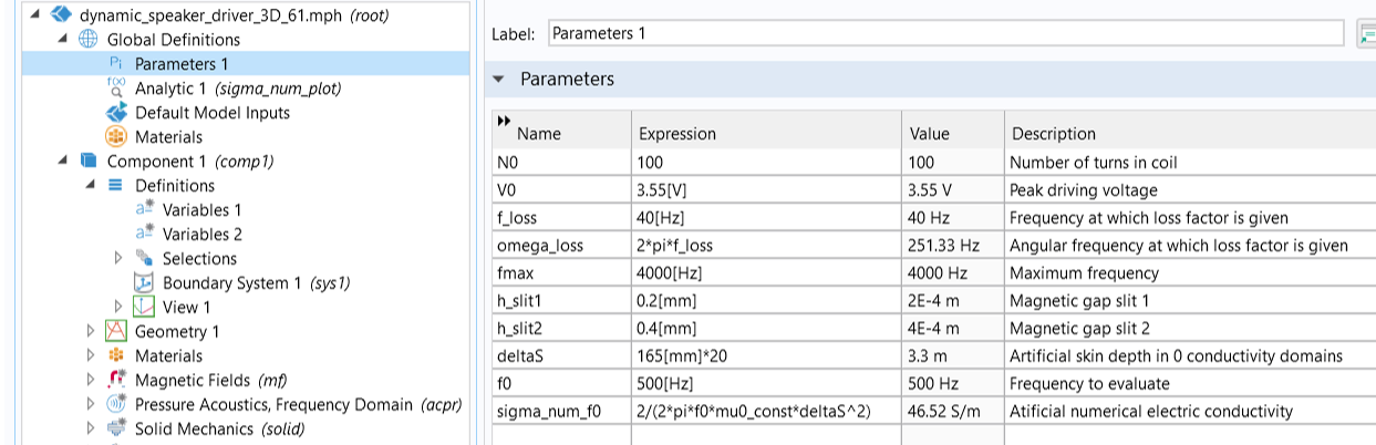A close-up of the Parameters node selected in the Model Builder and the Parameters table in the Settings window. 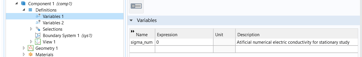A close-up of the Variables node selected in the Model Builder and the Variables table in the Settings window. A close-up of the Model Builder with a second Variables node selected and the corresponding Variables table in the Settings window.

Settings options for formulating a frequency-dependent artificial electrical conductivity for the perturbation analysis to improve the convergence of iterative solvers.

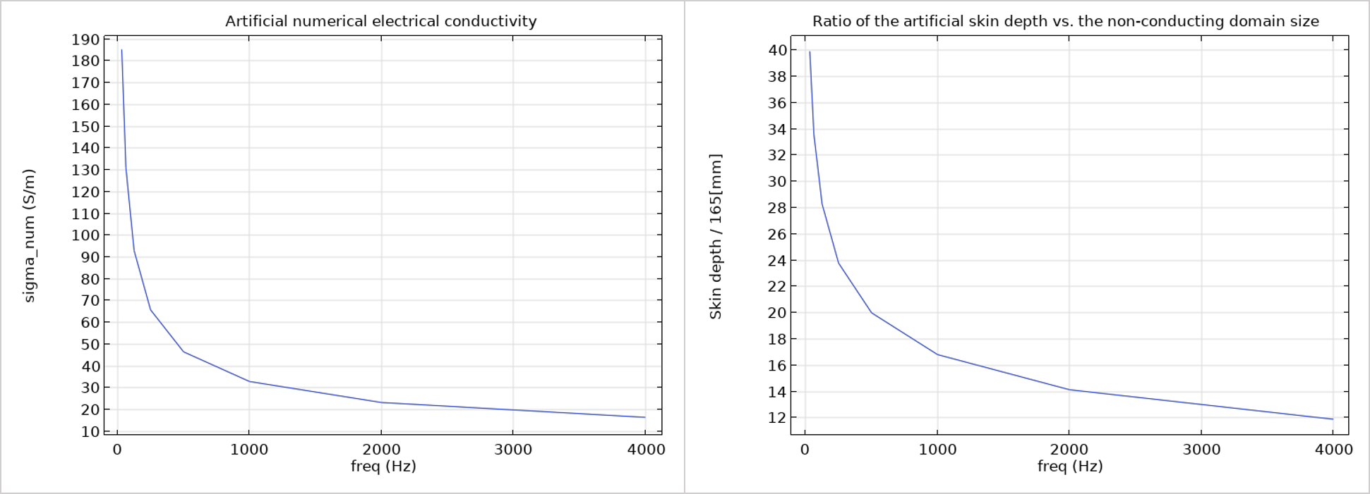
The curves below show the applied artificial electrical conductivity (left) and the ratio of the corresponding artificial skin depth versus the nonconducting domain size (right) as a function of frequency. You can see the skin depth is still more than 10 times of 165 mm for the highest study frequency. This ensures negligible induced current and thus negligible artificial electrical loss in these otherwise lossless domains for all study frequencies.

Two side-by-side graphs, with the first showing a dropping curve of the applied artificial conductivity that decreases quickly when frequency increases, and the one on the right showing the corresponding skin depth declining with frequency.

The applied artificial electrical conductivity (left) and the ratio of the corresponding artificial skin depth versus the nonconducting domain size (right) as a function of frequency.

The variablesigma_numis then used to define the electrical conductivity for all nonconducting materials in theMagnetic Fieldsinterface, as exemplified in the images below. This greatly improves the convergence of the iterative solver for lower frequencies.

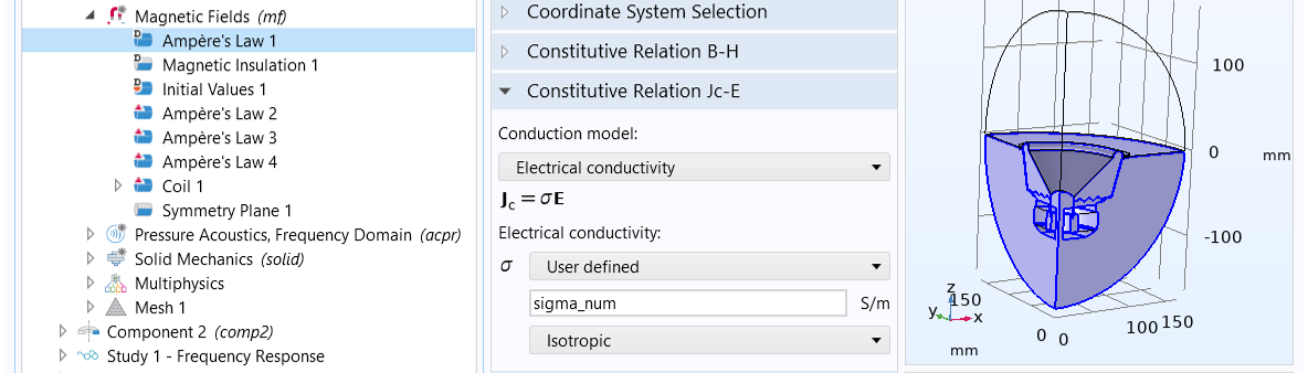A close-up of the Model Builder with the Ampère’s Law node selected and the corresponding Constitutive Relation Jc-E settings and model. 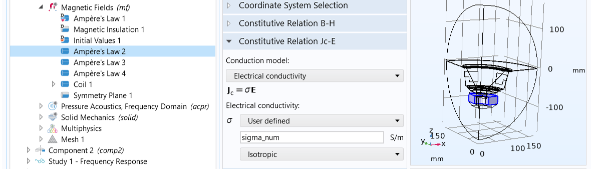A close-up of the Model Builder with a second Ampère’s Law node selected and the corresponding Constitutive Relation Jc-E settings and model.

Adding small electrical conductivity to all nonconducting materials greatly improves the iterative solver convergence for low frequencies.

Finally, select a variable definition forsigma_numat each study step so that zero electrical conductivity is used for the first two study steps and the frequency-dependent expression is used for the third perturbation study step. This is done by selecting theModify model configuration for study stepcheck box in thePhysics and Variables Selectionsection at each study step and disabling the unwantedVariablesnode, as shown in the images below.

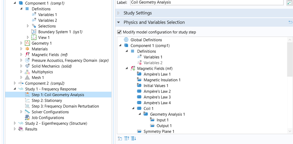A close-up of the Model Builder with the Coil Geometry Analysis feature selected and the Physics and Variables Selection in the corresponding Settings window, with the Modify model configuration for study step check box selected. 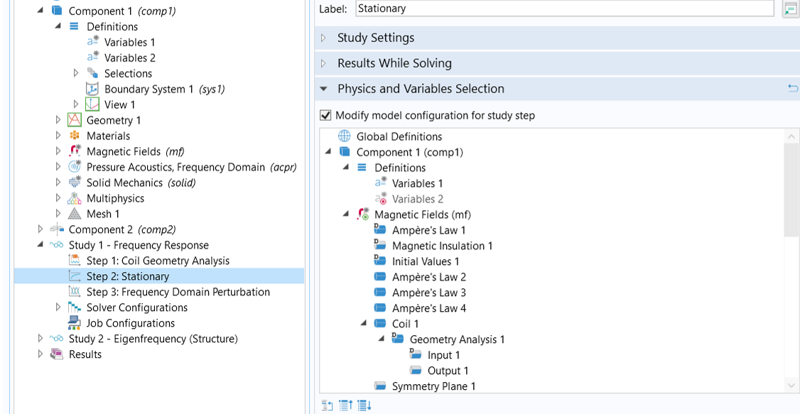A close-up of the Model Builder with the Stationary study step selected and the Physics and Variables Selection in the corresponding Settings window, with the Modify model configuration for study step check box selected. 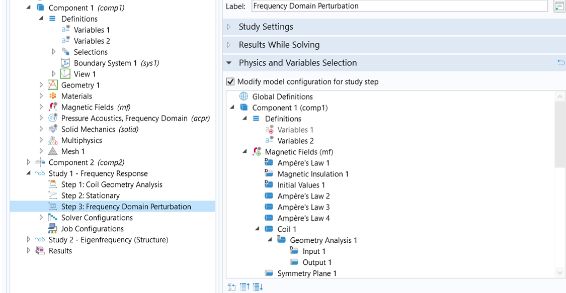A close-up of the Model Builder with the Frequency Domain Perturbation feature selected and the Physics and Variables Selection in the corresponding Settings window, with the Modify model configuration for study step check box selected.

Select a variable definition forsigma_numat the study steps so that zero electrical conductivity is used for the first two steps (top and middle images) and the frequency-dependent expression is used for the third step (bottom image).

Using the Autogenerated Iterative Solver

You can find the suggested solver options in the default solver settings. To show the default solver setup, right-click the study node and selectShow Default Solver, then expand the solver sequence, as shown below. The autogenerated solver suggestions include a direct solver (used by default) and an iterative solver (disabled). To switch to using the iterative solver, right-click the solver and selectEnable(or press F4).

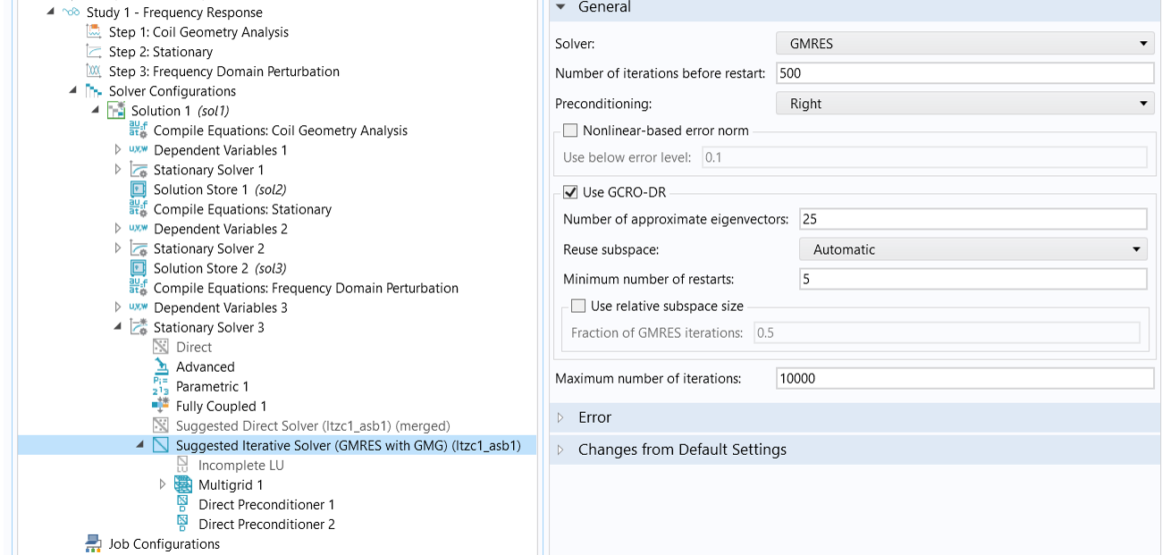A close-up of the Model Builder with the suggested iterative solver selected and the corresponding settings.

A suggested iterative solver is automatically generated and can be enabled for solving large models.

Further Learning

So far, we have discussed how to model a traditional dynamic speaker driver in the frequency domain. For the analysis of other types of speaker drivers, download the documentation and MPH-files from the Application Gallery (a link for the 3D dynamic driver example is also provided):

• Balanced Armature Transducer — Frequency-Domain Analysis
• Piezoelectric MEMS Speaker
• Electrostatic Speaker Driver
• Loudspeaker Driver in 3D — Frequency-Domain Analysis

Also seeSupplement B - More Information on Iterative Solvers for 3D Analysisfor additional information.