Finite Element Time-Dependent Analysis
In Part 1 of this course, we discussed the applicability of frequency-domain and time-dependent analyses. Let's recap the circumstances that require a transient model:
- The excitation is a short pulse or includes more than one frequency component.
- The problem becomes nonlinear. The nonlinearity can be due to large signal excitation and higher harmonic generation, a nonlinear magnetization model, or a geometry/topology change because of large deformation.
- The output of interest is the transient response to an excitation.
In this part of the course, we use the same dynamic speaker driver as in Part 2 (which focuses on a frequency-domain study) to discuss the specific considerations for running a transient analysis. The model is solved in the 2D axisymmetric space dimension, and the focuses of this study are to characterize the nonlinear behavior of the driver due to large deformation of the moving parts and to determine the total harmonic distortion (THD) of the acoustic signals produced by the system.
Geometry
The geometry for the transient analysis is shown below. The layer highlighted in blue is created for applying thePerfectly Matched Layerfeature in order to avoid unphysical reflections from the artificial boundaries added to form a finite-sized computational domain. ThePerfectly Matched Boundaryfeature used in Part 2 is only available in a frequency-domain pressure acoustics model. For time-domain simulations, use thePerfectly Matched Layerfeature, which is applied to a virtual domain attached to an open boundary.
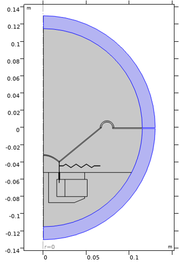
The geometry for a transient analysis. To apply the Perfectly Matched Layer feature to absorb outgoing waves, having a virtual domain attached to the open boundary is necessary.
The geometrical thickness of the perfectly matched layer (PML) in a geometry needs to be set adequately. The thickness can be determined by the following two meshing considerations:
- Use the same mesh element size as that in the adjacent physical domain
- Use a structured mesh with at least 6 mesh layers for the rational scaling and 8 for the polynomial scaling
The recommendation of using the same mesh size in both physical and PML regions is because of the implementation of PML in the time domain: There is no stretching with respect to the real coordinate in the PML, thus, the waves propagate through the PML with the same wavelength that they have in the physical region.
Required Physics Interfaces
Performing the transient analysis requires theMagnetic Fieldsinterface in the AC/DC Module and theAcoustic-Solid Interaction, Transientmultiphysics interface in the Acoustics Module. Note that COMSOL®has distinct physics interfaces that solve specific formulations of the wave equation in fluids for different types of analyses. It is therefore important to ensure that the correct physics interface is selected to match the study type. The following image shows the location of the transientAcoustic-Solid Interactioninterface in theSelect Physicswindow of the Model Wizard.
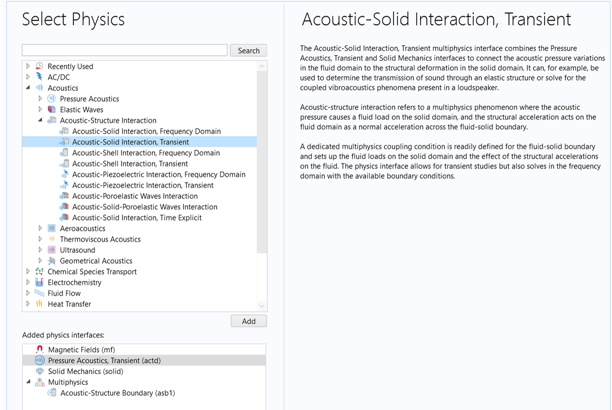 The Select Physics window with the Acoustic-Solid Interaction, Transient interface selected and a description of the feature.
TheAcoustic-Solid Interaction, Transientmultiphysics interface is under theAcoustics>Acoustic-Structure Interactionbranch of theSelect Physicswindow of theModel Wizard.
This feature combines thePressure Acoustics, Transientinterface, a transient acoustic model, and theSolid Mechanicsinterface. Similar to how we performed a frequency-domain analysis in Part 2, theAcoustic-Structure Boundarycoupling feature is automatically added to the model to connect thePressure Acoustics, Transientinterface with theSolid Mechanicsinterface. Later, aLorentz Couplingfeature should be manually added to theMultiphysicsnode in the model tree to couple theMagnetic Fieldsinterface andSolid Mechanicsinterface (in the same way as described in Part 2).
Using a Moving Mesh in a Transient Model
TheLorentz Couplingfeature is formulated differently for a transient analysis than that for a frequency-domain analysis. In the frequency domain, the formulation explicitly includes the back EMF contributions: It passes the Lorentz force from theMagnetic Fieldsinterface to theSolid Mechanicsinterface and passes the structural velocity that leads to the induced electric field from theSolid Mechanicsinterface to theMagnetic Fieldsinterface. However, in the time domain, only the Lorentz force is passed from theMagnetic Fieldsinterface to theSolid Mechanicsinterface, but the induced currents are not included in the formulation. You need to use a moving mesh in order to capture the back EMF contributions. This specific handling of transient analysis is to avoid double counting of the back EMF when one wants to use a moving mesh to capture nonlinearity due to large deformations and geometry/topology changes, like when the coil is moving partially or fully in and out of the magnetic gap. Since the induced currents are captured automatically by a moving mesh, including them in the coupling formulation will give wrong results.
Therefore, in transient studies it is always necessary to use a moving mesh even for small displacements, because the induced currents are only captured that way. In the current case, we are also interested in modeling the effect of structure deformations on the magnetic field and acoustic field, which adds another source of nonlinearity to the problem.
TheMoving Meshfeature can be added by clickingMoving Meshand choosingDomains>Deforming Domainin theDefinitionstoolbar, as seen in the image below.
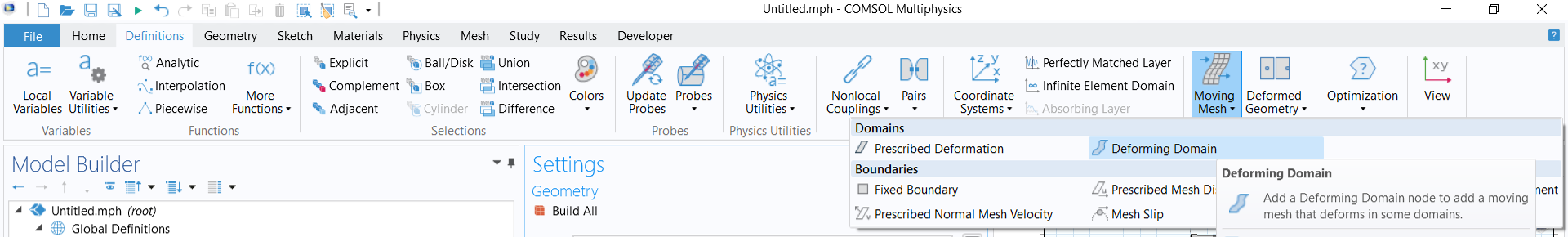 The top half of the COMSOL UI, with the Moving Mesh feature selected in the toolbar and the resulting options with Deforming Domain selected.
TheMoving Meshfeature can be added from theDefinitionstoolbar.
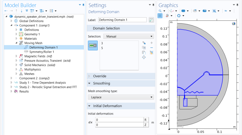
This adds aMoving Meshinterface to the model tree. The following steps are necessary in order to set up the moving mesh correctly:
- In theDeforming Domain 1subnode, select the air domains above and below the moving parts forDomain Selectionand chooseLaplacefrom theMesh smoothing type listforSmoothing, as seen in the image below. Once the deforming domains are specified, prescribed mesh displacements using the solid displacement components are automatically added to all boundaries next to a solid, and a fixed boundary is used for all other outer boundaries.
 The COMSOL Multiphysics UI showing the Model Builder with the Deforming Domain feature selected and the corresponding Settings window with Laplace selected for the mesh smoothing type.
TheLaplacemesh smoothing type is used in the deforming domains.
Compared to other nonlinear smoothing methods, theLaplacesmoothing is the cheapest option in terms of computations because it is linear and uses one equation for each coordinate direction, which are not coupled together. This method is suitable when the mesh deformation is not too large, and especially when it is used together with anAutomatic Remeshingfeature, which ensures a new mesh is created whenever the mesh quality becomes less than a given limit.
- Add aSymmetry/Rollerfeature to specify a symmetry condition on boundaries at r = 0. This allows the mesh to "slide" there.
 The COMSOL Multiphysics UI with the Symmetry/Roller feature selected and the corresponding settings and model.
TheSymmetry/Rollercondition is applied to boundaries lying at r = 0.
Time-Domain Perfectly Matched Layer Settings
The recommended values of the PML scaling factor and scaling curvature parameter are 1,3 for thePolynomialstretching type, and 1, 1 for theRationalstretching type. Here, we use thePolynomialoption, as shown in the image below.
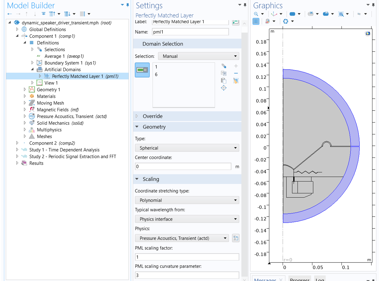 The COMSOL Multiphysics UI showing the Model Builder with the Perfectly Matched Layer feature selected, the corresponding settings, and the geometry with the outer layer highlighted in blue to show where the PML feature is applied.
ThePerfectly Matched Layersettings for the transient analysis.
Input Signal for Transient Analysis
Performing a transient analysis of the speaker requires a time-dependent voltage signal,V(t), applied to the voice coil. The choice of a specific type of input signal depends on the characteristic under investigation. In this case, the input is a harmonic voltage signal:

The input signal frequency and the amplitude are chosen asf0=70HzandV0=10V, respectively.
When solving a transient model, it is good practice to ramp up the load to minimize numerical error. An instantaneously applied load leads to a lot of high-frequency content generation due to the inertia effect of the system it applies to, and when they are unresolved, numerical error or even solver divergence can occur. This is also physically motivated since most loads cannot truly change instantaneously in time. You can use aSteporRampfunction with appropriate smoothing for this purpose.
In this analysis, we use the driving signal period,T0=1/f0, to define a ramp function,rm1(t), that has a slope of1/T0. The ramped input signal,V0*sin(2πf0t)*rm1(t), is then used to define the coil voltage, as shown in the image below. This allows the load to take one period to reach its full magnitude.
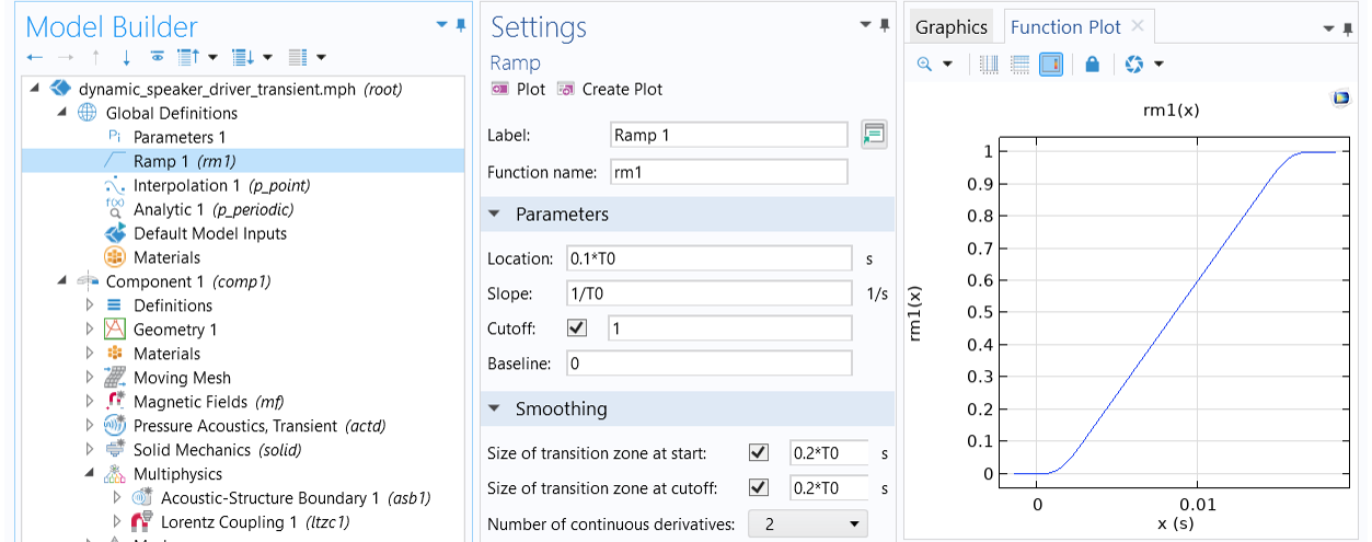 The Ramp function selected in the Model Builder, the corresponding Parameters and Smoothing settings, and the function plot.
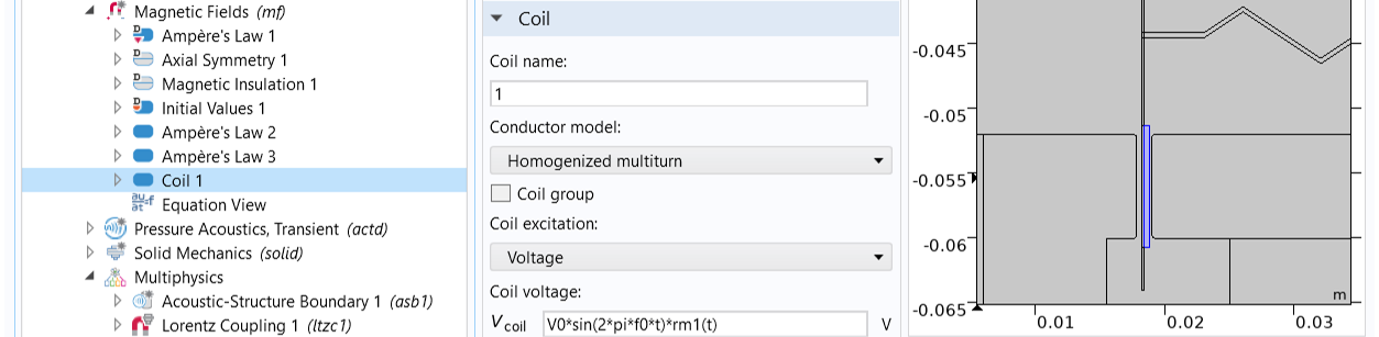 A close-up of the Coil feature selected in the Model Builder and the Coil section of the corresponding Settings window, with a close-up of the model in the Graphics window.
ARampfunction is defined using the driving signal period (top), and is then used to smooth the input signal (bottom).
Time Stepping Control Setup in Physics Settings
When solving transient models, you should first determine the maximum frequency you want to resolve (known asfmax). Enter the value of the maximum frequency into theMaximum frequency to resolvefield in theTransient Solver and Mesh Settingssection of thePressure Acoustics, Transientmain physicsSettingswindow, as shown in the image below. TheTime steppingsetting can also be found in this section, enabling you to set the time-stepping method as eitherFixed (preferred)orFree. In this case, it is recommended that you use theFixed (preferred)method, which is best suited for handling wave propagation. With the settings shown here, the autogenerated solver will be sufficient in most scenarios provided that the computational mesh also resolves the model's frequency content. Here, we setfmaxto3f0to capture up to the 3rdharmonic.
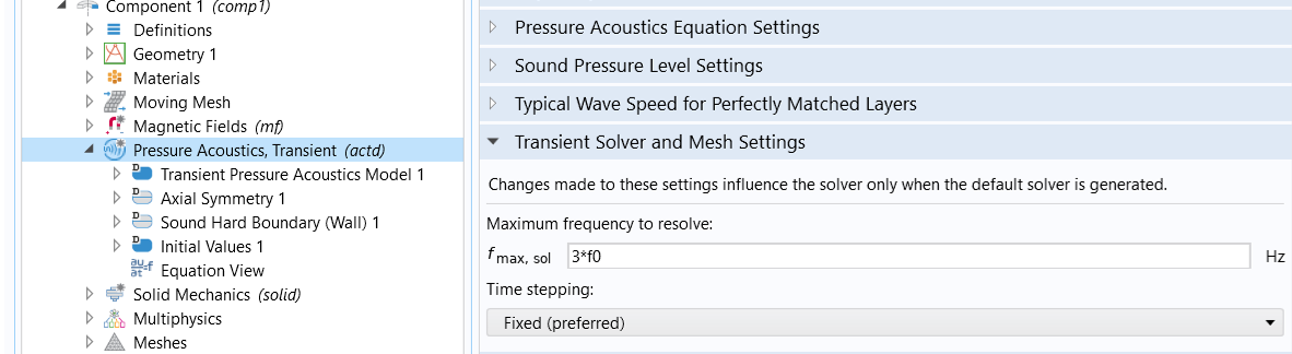 A close-up of the Pressure Acoustics, Transient feature selected in the Model Builder and the corresponding Settings window showing the Maximum frequency to resolve and Time stepping settings.
The transient solver settings at the top physics level.
Study Steps
Similar to the frequency-domain analysis, the transient study is also carried out using two study steps. First, aStationarystep is used to solve only the electromagnetic part of the problem in order to evaluate the field of the permanent magnet, with the driver in standstill. Then, the fullTime Dependentstudy step takes care of all the relevant multiphysics interactions of the moving speaker.
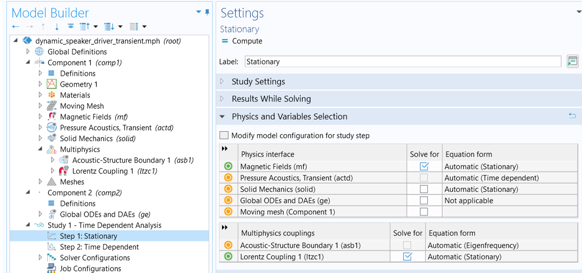 The Stationary Study selected in the Model Builder and the corresponding Settings window showing the tables in the Physics and Variables Selection setting.
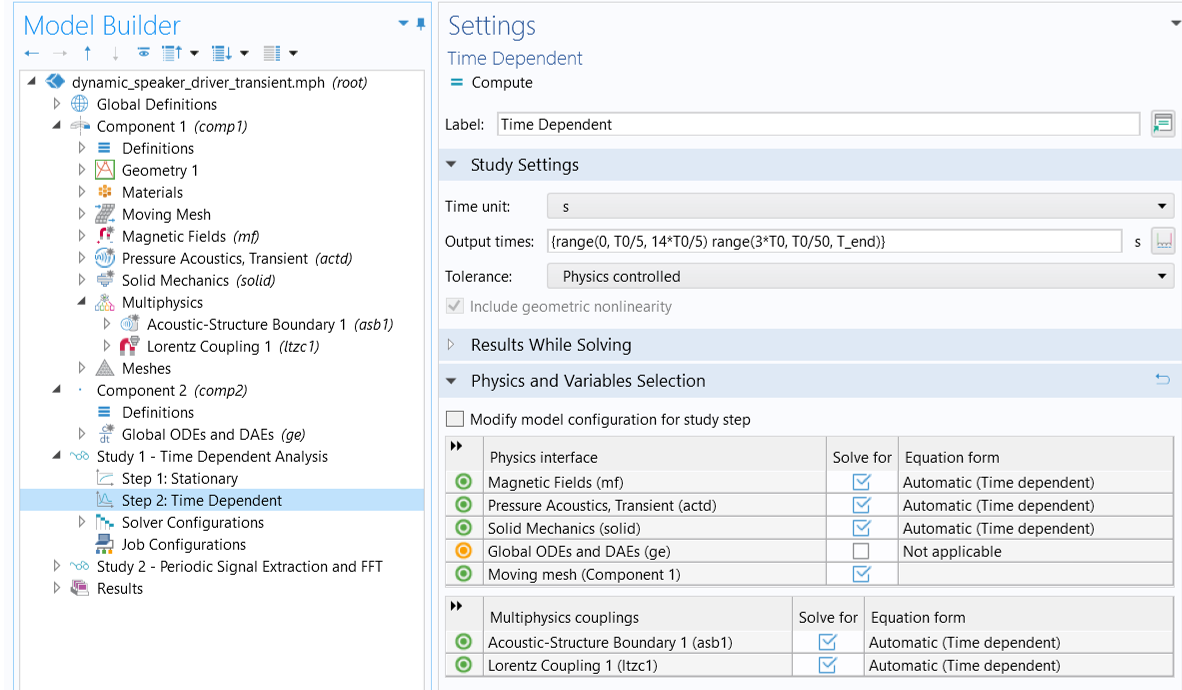 The Time Dependent study selected in the Model Builder and the corresponding Settings window showing settings such as the output times and physics and variables selection.
Study step settings for transient analysis.
TheTime Dependentstudy step solves for the period of time from0toT_end = 4T0. The full output time range is split into two subintervals: from0to3T0and from3T0toT_end. The second subinterval is of the most interest since it is assumed that the steady state takes place from time3T0. Therefore, the output time stepping is finer over the second subinterval in order to obtain a steady-state solution with better time resolution.
TheAutomatic remeshingoption is enabled in theTime Dependentstudy step to avoid using highly distorted meshes, which could lead to numerically ill-posed problems. In this model, a new mesh is created as soon as the distortion of the current mesh elements exceeds a certain level, which you specify in advance.
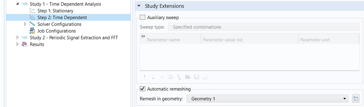 A close-up of the Time Dependent study selected in the Model Builder and the Study Extensions settings in the corresponding Settings window.
TheAutomatic remeshingoption is enabled in theStudy Extensionssection of theTime DependentstudySettingswindow.
Here are the steps for specifying the condition for remeshing:
- ClickShow Default Solverin theStudytoolbar.
- Expand the solver sequence and clickAutomatic Remeshingunder theTime-Dependent Solver 1node.
- In theCondition for Remeshingsection of theSettingswindow forAutomatic Remeshing, chooseDistortionfor theCondition typeand enter2.5in theStop when distortion exceedstext field, as seen in the image below.
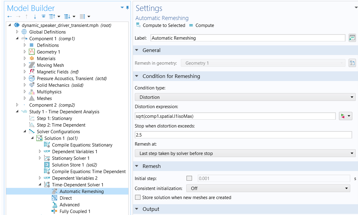 The Automatic Remeshing feature selected in the Model Builder and the corresponding Settings window showing the Condition for Remeshing settings, such as Distortion set as the condition type.
TheCondition for Remeshingsetup.
This condition ensures that the solver remeshes when the square root of the maximum element distortion, stored in the variable namedcomp1.spatial.I1isoMax, becomes larger than 2.5.
As seen in the image below, in theTime Steppingsettings, the default transient solver uses the input value of theMaximum frequency to resolvesetting to resolve up to the maximum frequency component.
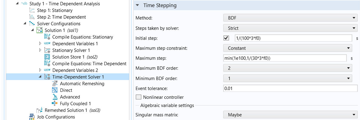 The Time-Dependent Solver selected in the Model Builder and a close-up of the Time Stepping settings in the corresponding Settings window.
Time stepping used by the autogenerated solver.
Initial Mesh
We need an initial mesh to start with, and a new mesh will be automatically generated whenever the mesh distortion tolerance is reached.
For transient models, the mesh needs to be able to resolve the maximal frequency you want to capture, sayfmax. This frequency translates to a minimal wavelength,λmin=c/fmax, and in turn to a maximum element size,hmax<λmin/5. Use this criteria to determine the maximum element size for each domain.
The initial mesh is seen in the image below. It usesMappedmeshes for the thin solid domains, including the coil, former, spider, cone, and suspension, andFree Triangularmeshes for the rest of the physical domains.Mappedmeshes with a distribution of 8 elements are applied to discretize the PML domains. Refer to the attached MPH-file for the detailed meshing sequence.
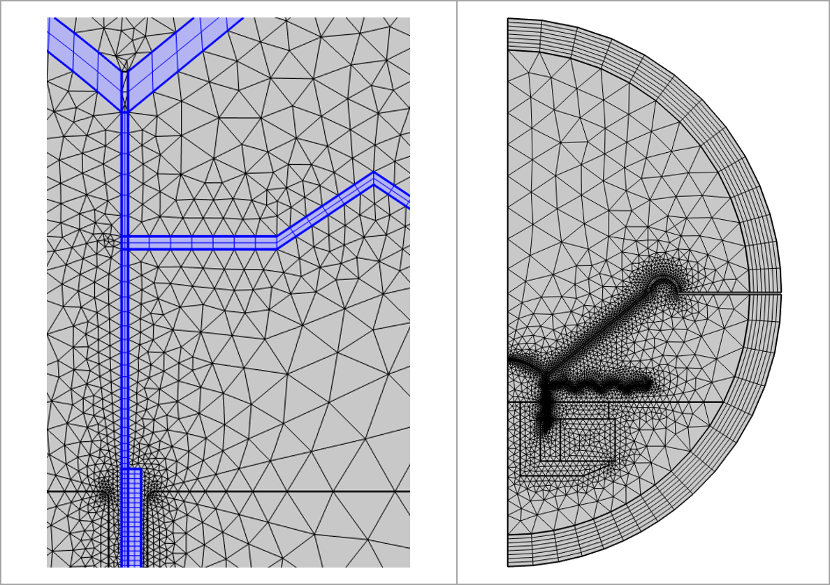 A close-up of the initial mesh and the mesh of the half-circle.
The initial mesh used for the transient analysis.
The present model runs at a relatively low frequency (including the harmonics) and does not require a resolution of eddy currents (the skin depth) in the pole piece. Thus, compared to the frequency-domain analysis, the boundary layer mesh has been removed.
Transient Solutions and Analysis
The animation below shows the magnetic field in and around the voice coil gap, the motion of the voice coil (orange), the former, the spider, and the cone (pink), as well as how the moving mesh adapts the mesh to the changed topology of the system during the time period of3T0to4T0.
Magnetic field in and around the voice coil gap and the motion of the moving parts and mesh deformation during the time period of 3T0to 4T0.
The plot below depicts the relative position of the voice coil, calculated as the vertical displacement from its original position averaged over the coil domain. The voice coil is at the lowermost position at 0.044 s (the green marker). At 0.048 s (the red marker) and 0.052 s (the cyan marker), the coil is on its way up and down, respectively.
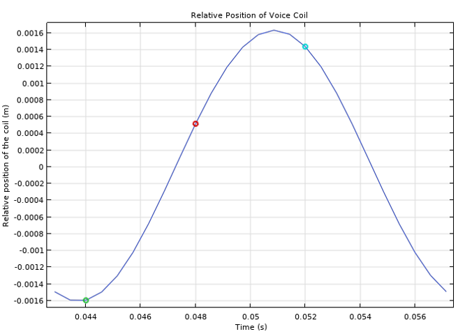
Relative position of the voice coil.
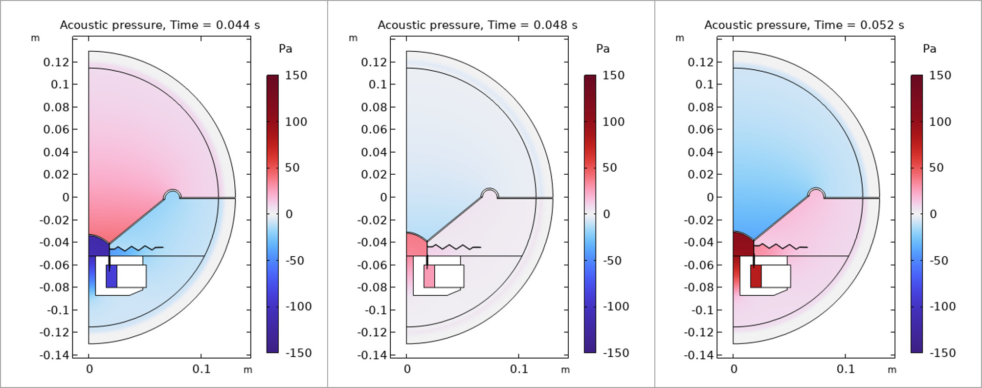
The distribution of the acoustic pressure around the speaker driver at these three time steps — 0.044 s (left), 0.048 s (middle), and 0.052 s (right) — are shown in the figure below. You can also see how the PML attenuates the acoustic waves generated by the motion of the speaker cone.
 Three side-by-side images showing the acoustic pressure at different time steps.
Acoustic pressure at 3 different time steps.
Total Harmonic Distortion (THD) Calculation
An important output of interest of this analysis is the total harmonic distortion of the acoustic signals produced by the system. Distortion analyses, including the total harmonic distortion (THD) and intermodulation distortion (IMD), are commonly used to judge the quality of a speaker driver. These nonlinear effects produce overtones and additional nonharmonic frequency components, the extent of which can be quantified and calculated using the approaches discussed in our blog post "How to Perform a Nonlinear Distortion Analysis of a Loudspeaker Driver". To calculate THD, we first need to choose a point of interest as a listening point, and obtain the frequency spectrum of the steady-state acoustic pressure at this listening point. The value of THD is then calculated as
 ,
,
whereH{sub}Nis the harmonic response of the Nthharmonic andH1is the fundamental response.
Here, we choose the listening point at r = 0 and z = 0.115 m, the highest point in the physical domain lying on the acoustic axis. It is assumed that the speaker reaches the steady state by timet=3T0, and therefore the pressure signal as a function of time fromt=3T0tot=4T0at this specific listening point is the steady-state solution that can be used for THD calculation, as seen in the plot below. You can see that the profile slightly differs from a perfect sinusoidal. This means that the output signal also contains frequency components other thanf0.
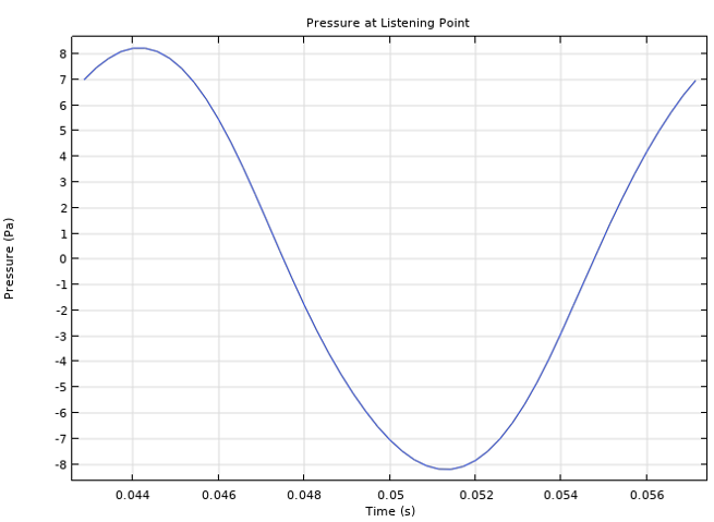
Acoustic pressure at the listening point.
Note that the accuracy of the FFT computation becomes higher for longer time intervals. Therefore, in order to obtain more accurate frequency spectrum of this one cycle signal, we perform a periodic extension of the data over time. This is done by the following steps:
- Use aPoint Evaluationfeature to evaluate the pressure at the listening point from3T0to4T0with a time step ofT0/50. This creates a table that stores the acoustic pressure as a function of time. See thePressure at Pointnode underResults>Derived Valuesin the attached model file.
- Define anInterpolationfunction using theResult tableas the data source and the table created from Step 1. The signal is interpolated by a cubic spline. See theInterpolation 1 (p_point)node underGlobal Definitions.
- Define anAnalyticfunction using the interpolation function specified in Step 2 and make it periodic through thePeriodic Extension. See theAnalytic 1 (p_periodic)node underGlobal Definitions. The extended pressure signal is seen below.
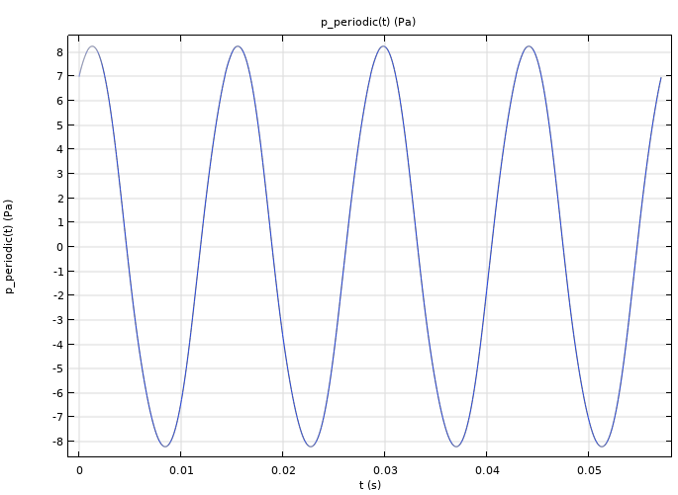
A periodic extension of the pressure signal at the listening point.
The frequency spectrum analysis of the extended signal is then taken care of by theGlobal ODEs and DAEsinterface defined inComponent 2and the second study, as seen in the images below. The study here consists of aTime DependentandTime to Frequency FFTstep. The first study step solves a global equation that passes the values of the periodically extended signal to a dependent variable namedP; the second study computes the FFT ofP. The first step is necessary because aTime to Frequency FFTstudy performs a forward FFT on only a dependent variable that an interface solves for. Here, we choose to extend the signal to 10 acoustic cycles for more accurate FFT computation.
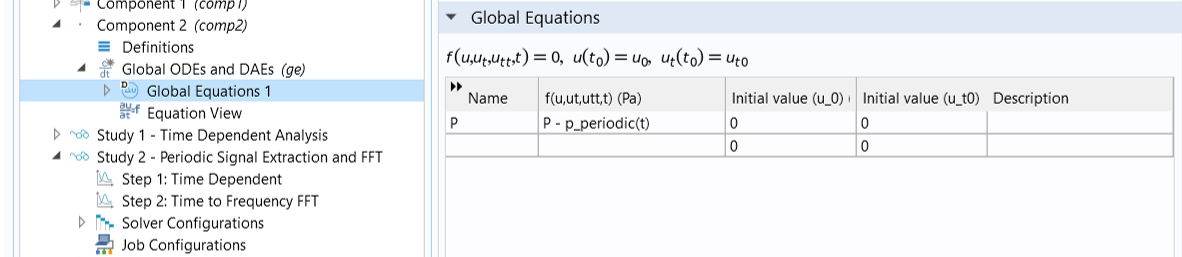 A close-up of Global Equations selected in the Model Builder and the corresponding Settings window with the Global Equations table for variable P.
The periodic extension of the pressure signal is passed onto a dependent variable,P,solved by aGlobal ODEs and DAEsinterface.
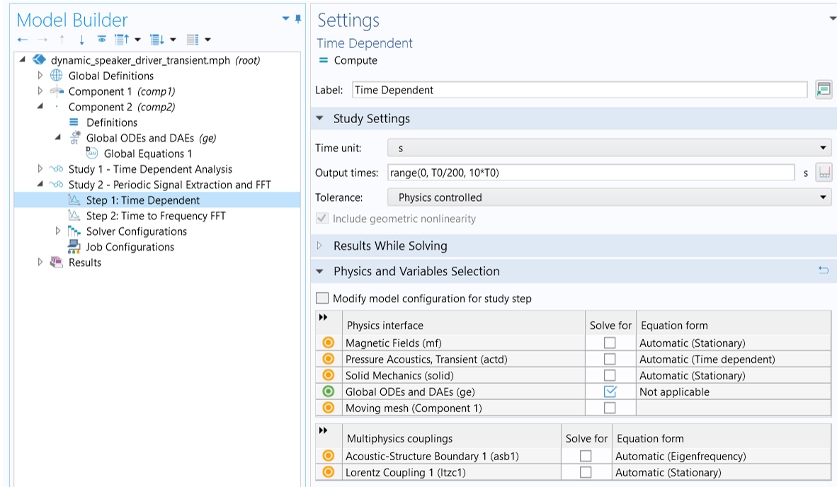 The Model Builder with the Time Dependent study selected and the Settings window showing the Study Settings and Physics and Variables Selection table.
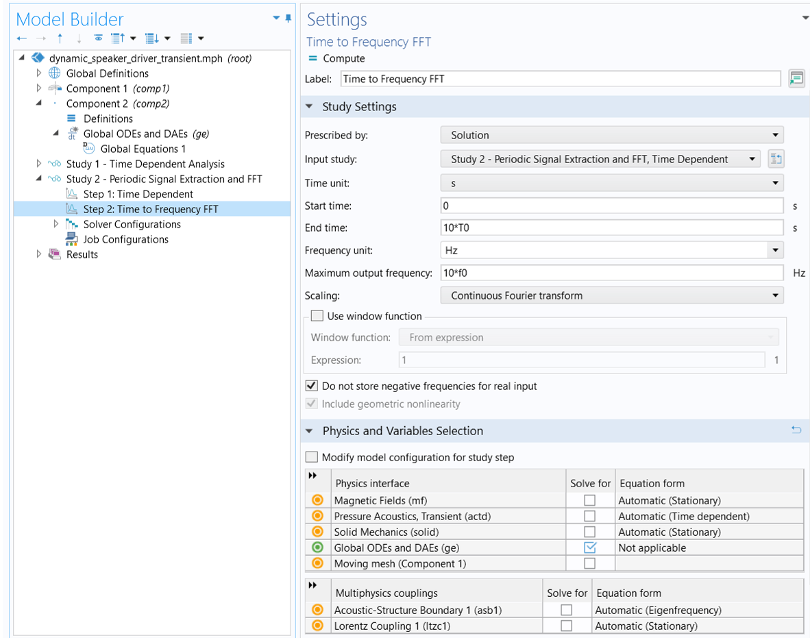 The Model Builder with the Time to Frequency FFT study selected and the Settings window showing the Study Settings and the Physics and Variables Selection table.
Study steps used for the frequency spectrum analysis of the extended signal.
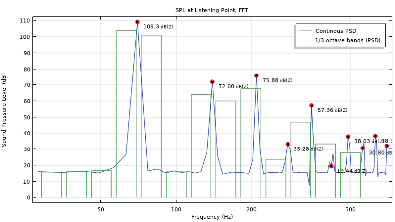
The figure below shows the frequency spectrum of the acoustic signal obtained from the FFT study as the value of SPL over frequency. The highest peaks appear at frequencies that are multiples of f0(red dots), and it is notable that the SPL for the odd-order harmonics is higher than that for the even-order harmonics, which means the symmetrical system nonlinearities dominate the asymmetrical ones.
 A graph showing the 1/3 octave bands (PSD) as green bar graphs and the continuous PSD as a blue line, with both lines peaking after 50 Hz.
The frequency spectrum of the acoustic signal (represented as SPL over frequency) at the listening point.
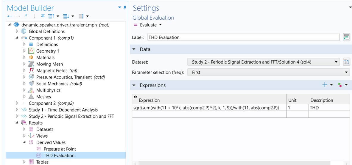
The THD value is computed inDerived Values>THD EvaluationusingGlobal Evaluationwith the following expression:
sqrt(sum(with(11 + 10*k, abs(comp2.P)^2), k, 1, 9))/with(11, abs(comp2.P))
 The Model Builder with Global Evaluation selected and the corresponding Settings window showing the dataset data and the calculated expression.
THD calculation usingGlobal Evaluation.
The expression uses thewithoperator to access the solution of a specific frequency component and thesumoperator to compute the sum of the expressions for all index values. More specifically,with(11, abs(comp2.P))provides the acoustic pressure amplitude for the fundamental frequency (the 11thoutput frequency is 70 Hz), andsum(with(11 + 10*k, abs(comp2.P)^2), k, 1, 9), wherekis the summation index, calculates the sum of the squared pressure amplitude of the first 9 harmonics. If you take a look at the output frequencies from the FFT study, you will see the index corresponding to the fundamental frequency and its harmonics. Such a calculation of including 9 harmonics yields a THD equal to 2.5%.
Further Learning
This tutorial model and detailed documentation with step-by-step analysis instructions are also available for download in the Application Gallery:Loudspeaker Driver — Transient Analysis.
请提交与此页面相关的反馈,或点击此处联系技术支持。