学习中心

Modeling with PDEs: Using the Weak Form for Equation Systems

---

In Part 11 of this course, we will go deeper into techniques for setting up partial differential equations (PDEs) in COMSOL Multiphysics^® using the weak formulation of the equations. Specifically, we will look at coupled systems of equations. To illustrate this, we will continue from the plane stress example in Part 9 and compare using the built-in interface for plane stress with a user-defined plane stress equation system defined using the Weak Form PDE interface.

The Weak Form of the Equations for Linear Elasticity

In Part 9, we saw how to implement the equations for plane stress using the Coefficient Form PDE interface. Here, we will go over how to derive the corresponding weak form. To do this, we can start by looking at the general 3D case for linear elasticity.

Hooke's law for a potentially anisotropic, linear elastic material can be written as:

if we use the so-called Einstein summation convention, where we sum over indices that occur twice in an expression. The expression above is shorthand for:

with the added benefit that we do not need to write out the summation signs.

Just like in Part 9, we will keep things simple and assume small deformations as well as small rotations. The notation used in Part 9 is related to this notation in the following way:

The stress tensor components:

...

The strain tensor components:

...

The tensor-valued material coefficient:

is the stiffness, or elasticity, tensor.

The dependent variables in 3D are for the displacements in the x, y, and z direction, respectively.

The strains are related to the dependent variables as:

and so on.

Following the energy approach of Part 10, when solving a linear elasticity problem, the corresponding minimization problem is to minimize the total potential energy in a system, which consists of the internal elastic energy as well as the potential of the loads. We will now consider a computational domain with boundary . Using the notation discussed here, the potential energy can be written as:

Here, the are the components of the surface traction vector.

For simplicity, we will assume that there are no body forces.

The first variation is:

There are plenty of symmetries in the stiffness tensor. For instance, we have the following relationships:

Using these symmetries and Hooke's law, we can rewrite the first term as:

So, the condition for stationarity is:

This general formulation is also valid without the assumption of linear elasticity. One reasons for this is that in the volume term we are not applying the variation operator directly on the dependent variables, but on the strain. (This is true as long as we are using stress and strain definitions that are "conjugate" or "compatible".) This format enables us to use a much more compact notation, which is one of the benefits of working with the weak form. Note that in structural mechanics, this form of the equation is also known as the principle of virtual work.

Recall that when we write a test function component such as:

we implicitly are using the fact that since:

we also have that:

(together with the condition for admissibility).

In general, we have:

or, using vector notation:

and

Using tensor notation, we can write

as

where symbolizes a suitable tensor product with summation over two indices.

Similarly, we can write the boundary term

as

Now, by using

the weak form of the equation becomes

Just like in Part 10, we can perform partial integration to get back to the strong form of the equation, or the system of equations:

Note that since is a vector, we have that:

meaning that we can write the equation as:

The quantity

is the force per unit area on the boundary with unit normal vector . It also corresponds to the Neumann boundary condition:

This means that we are left with just the domain integral term for a problem with only Neumann boundary conditions.

The domain integral:

needs to be valid for all admissible choices of the test functions

The only way for this to happen is if:

This is Navier's equation from Part 9, for a problem with Neumann boundary conditions for the boundary load.

In the presence of a body force, or load, , we instead get:

If we include a body force in the weak form we get:

Note that the weak form equation is a scalar-valued equation, due, in part, to its relationship with energy, whereas Navier's equation is vector valued. The weak form of a PDE is always scalar valued, but, in the case of two or more dependent variables, the strong form is not.

The Weak Form Equation for Plane Stress

For plane stress, we saw in Part 9 that the relationships between the stress and strain tensor components are described by:

with all other stress components equal to zero.

However, note that is not zero since

but the variation of does not enter the weak form since .

For more information on the relationships between the stress and strain components for plane stress, see our blog post on the difference between plane stress and plane strain.

We can now put the plane stress equations in the weak form as the integrand for the domain part of the integral:

where we have moved the integral to the right-hand side, following the convention used in the Weak Form PDE interface.

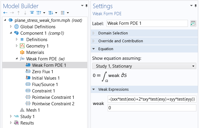
The weak form equations for plane stress under the Weak Form PDE node for a model.

Only some of the terms are nonzero, so, in practice, for the domain integrand we get:

But, due to symmetry, we have that

and

so, we can write the domain part of the weak form expression as:

or, using the other equivalent notation:

In the case of a surface stress boundary condition, the boundary terms are:

However, in the plane stress case the last term is ignored.

Note that if we have the special case of a pressure load

we get:

or, in the 2D case:

A Rectangular Plate with a Circular Hole, Using the Weak Form PDE Interface

To set up the Weak Form PDE interface for plane stress, you go through the same steps in the Model Wizard as for using the Coefficient Form PDE interface, as shown in Part 9. We will also, as in the Coefficient Form PDE example, assume that we have the global parameters shown in the image below.

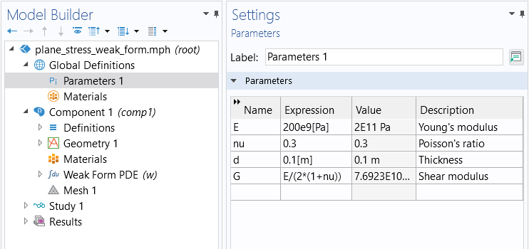
Global parameters for the weak form example.

Furthermore, we will assume that we have defined variables for the stress and strain components according to the figure below.

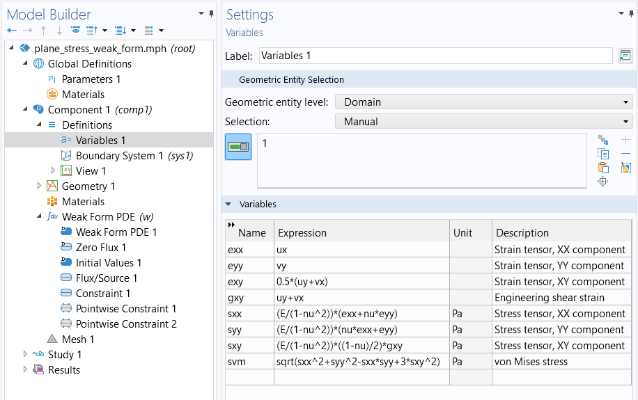
Variables for the stress and strain components for plane stress.

Using these definitions, we can enter the domain-level weak form equation as:

-(sxx*test(exx)+2*sxy*test(exy)+syy*test(eyy))

The figure below shows how this appears in the Weak Form PDE interface.

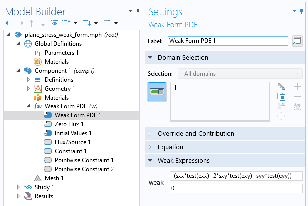
The weak form expression in the Weak Form PDE interface.

We use the same set of boundary conditions as in the example in Part 9. The Constraint and Pointwise Constraint conditions are identical. To enter the load on the rightmost boundary, there are several boundary conditions we can choose from. The simplest option is to use a Flux/Source boundary condition, as shown in the figure below.

The COMSOL Multiphysics UI showing the Model Builder with the Flux/Source boundary condition selected, the corresponding settings, and the Graphics window showing the rectangular plate. Entering the pressure load as a Flux/Source boundary condition.

Another way to enter the pressure load is to enter it as a weak contribution using the expression:

1e6*test(u)

as shown in the figure below. Weak contributions are discussed in more detail in the next few sections.

The COMSOL Multiphysics UI with the Weak Contribution node selected, the corresponding Settings window, and the Graphics window showing the rectangular plate. The settings for the Weak Contribution node.

To enter a load on a boundary with a general traction force, you can use an expression such as:

fx*test(u)+fy*test(v)

or, if the load is a pressure load:

-p*(nx*test(u)+ny*test(v))

Just like in the example in Part 9, the mesh setting used is Extremely fine. After computing, you can plot the various strain and stress components, and the results are identical to those implemented using the predefined physics interface versus the Coefficient Form PDE interface.

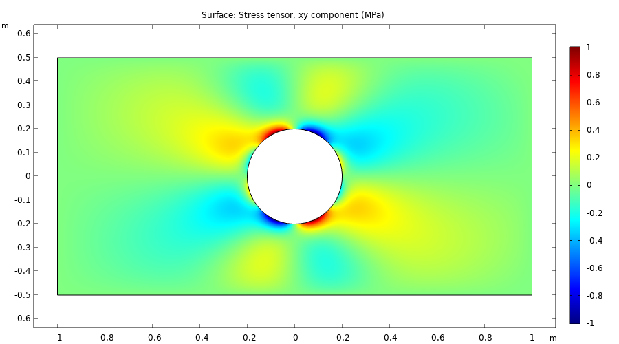
The stress component, sxy, visualized.

The Equation View Window

Notice that you get two Weak Expression text fields for entering the equation, but that we only use one of them. You can just as well enter some terms in the first field, and some other terms in the second field, since the terms will be summed up when forming the final weak expression that the solver will use. There are cases when having two Weak Expression rows are useful, such as when you want to use different integration orders for different parts of the equation system.

To see the integration order settings you need to enable the Equation View in the Show More Options dialog box that you open from the Model Builder toolbar. The Equation View nodes then appear in the model tree, as shown in the figure below.

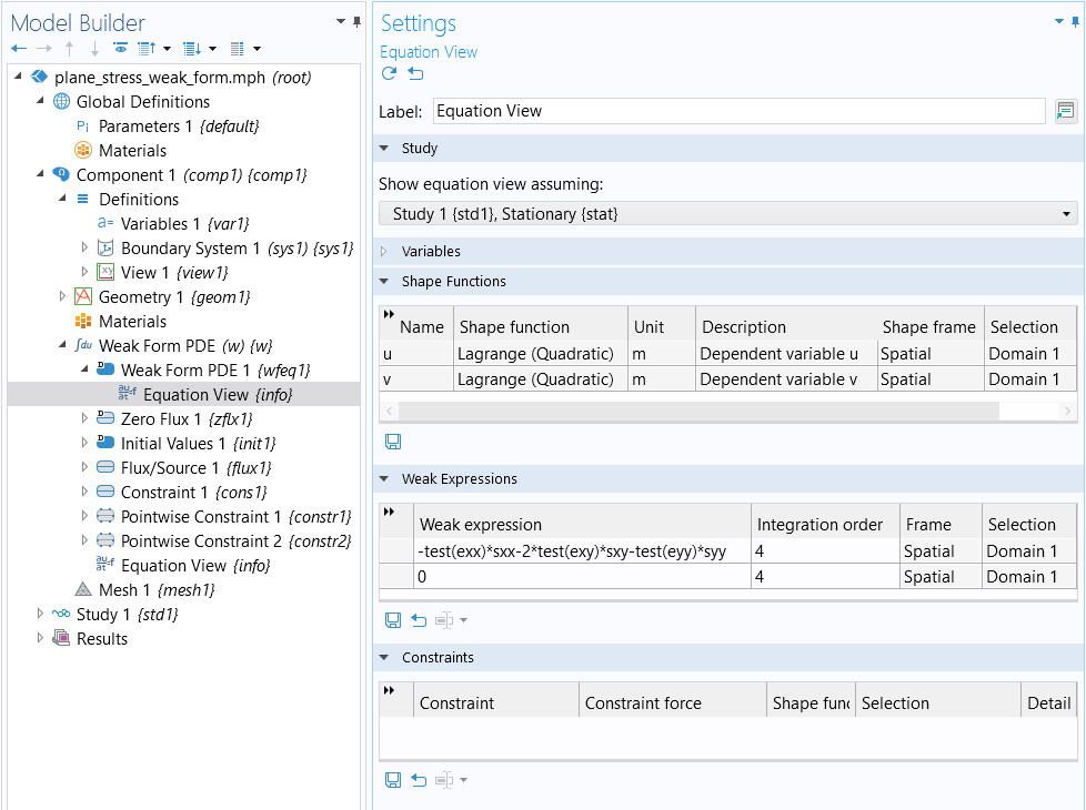
The integration order settings for a system of PDEs.

To learn more about numerical integration, see our blog post "Introduction to Numerical Integration and Gauss Points".

In the Equation View window, in the Weak Expressions section, you can see the weak form equations used by the interface. Each feature node of an interface has a corresponding Equation View window. This is also the case when working with the built-in physics interfaces. The Equation View window lets you "peek under the hood" and see both variable definitions (for example, strain and stress variables) as well as a listing of the weak expressions used.

Modifying the Equations and Weak Contributions

You can even add to, or modify, the weak terms in order to alter the underlying PDEs — including boundary conditions — of a built-in interface. To see an example of this, you can inspect the Equation View nodes in the thermal microactuator tutorial model. This model is available in the Application Libraries under COMSOL Multiphysics>Multiphysics, as shown in the figure below.

The thermal actuator tutorial model is available in the software through the Application Libraries.

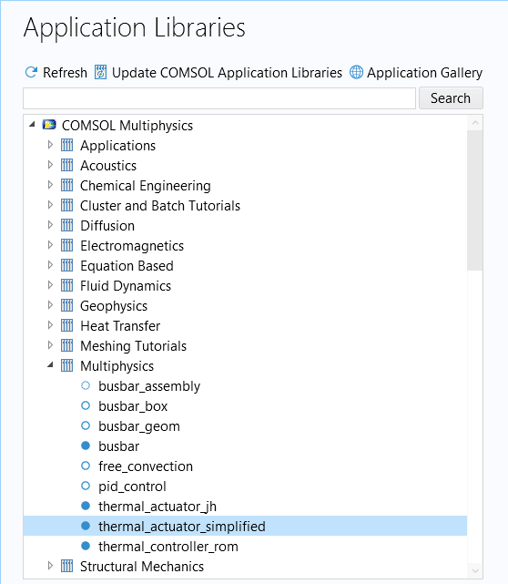
In this example, thermal expansion is implemented by modifying the corresponding variable definition for the strain tensor, as shown in the figure below. This process is detailed step by step in our Learning Center article on defining multiphysics models manually with user-defined couplings.

The Model Builder with the Equation View node selected and the corresponding Settings window showing the Variables table. The Equation View node where the changes have been made to the expressions for variables that define the strain tensor.

You can even modify the weak formulation of the predefined interfaces by adding weak contributions. To do so, you need to enable Equation-Based Contributions in the Show More Options dialog box. You will find this option alongside other advanced options in the context menu for the physics interfaces under More, as shown in the figure below.

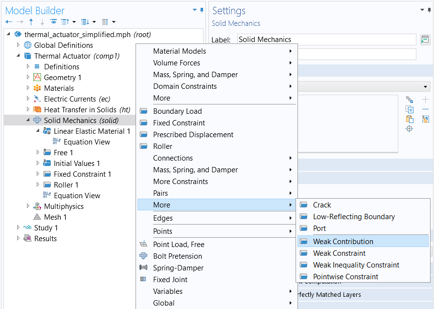
The context menu showing where to access the Weak Contribution node.

This will enable you to add additional equation terms, on the weak form, that describes extensions and modifications to the original equations. In the figure below, a weak contribution has been added to the equations for generalized plane strain; see also our blog post on modeling generalized plane strain. Note that since COMSOL Multiphysics^® version 5.3a, generalized plane strain is available as a built-in interface in the Structural Mechanics Module and the MEMS Module.

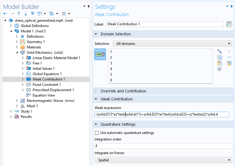
The settings for the Weak Contribution node.

The Weak Form for More General Physics

Not all types of physics stem from an energy minimization principle, but instead correspond to saddle points (which are still stationary points). A typical example of this is physics involving convection, such as the convection–diffusion equation or the Navier–Stokes equations.

In the case of the convection–diffusion equation:

with a Neumann boundary condition

we can derive the weak form by multiplying with a test function and integrate:

Next, perform partial integration:

then, using the boundary condition, we get:

As is conventional when using COMSOL^®, we move the equation to the right-hand side and get:

Note that in the domain integral the diffusive term is symmetric with respect to the test function and the dependent variable in the sense that they occur with the same order derivative. This is not the case for the convective term. This is a common characteristic of a weak form equation that does not have an associated energy. In the finite element discretization, this asymmetry of convective equation terms typically leads to nonsymmetric stiffness matrices. For more information, browse our blog posts on the weak form.

Different Ways of Using the Weak Form PDE Interface

You do not need to derive a weak form equation starting from a PDE or an energy expression; you can use a more direct approach. In the simplest case, you can intuitively consider the expression that the test function, such as test(u), is multiplied with as an equation that is set to zero, in the weak sense. In other words, if we, in the Weak Expression text field, for example, enter an expression such as:

test(u)*(u-f(x,y))

then this can be interpreted as the equation:

(u-f(x,y))=0

in the weak sense, as described earlier. Recall that an equation in the weak sense allows for discontinuities.

In the expression above, f(x,y) can be an interpolation function or an analytical function. The dependent variable field u will approximate this function using finite elements and, for example, piecewise polynomials defined on triangles or, in 3D, tetrahedra.

In this particular case, we can see that the weak form comes from the minimization of:

(u-f(x,y))^2

The stationary point is found by forming the first variation:

test((u-f(x,y))^2)=2*((u-f(x,y)))*test(u)

or in mathematical terms:

This should be understood as analogous to the chain rule:

Expanding on this, you can add test functions of the gradient of the dependent variable to introduce diffusive or convective effects, and so on. For an example where the derivation does not start from a PDE, see our blog post on image denoising and other multidimensional variational problems.

Further Learning

Although the model used as an example throughout this article is available for download, we encourage you to build the model yourself following the guidance provided here. This will help reinforce how to set up PDEs in the software using the weak form of the equations. You can open and investigate the file for the model example and compare it with implementation using the predefined physics interface.