学习中心

Modeling with PDEs: Vector- and Tensor-Valued Systems of Equations

---

In Part 9 of this course on modeling with partial differential equations (PDEs), we will learn more about setting up systems of PDEs. In particular, we will look at cases where the dependent variables represent the components of a vector or tensor field, such as the displacement vector and displacement field components in structural mechanics. These equations can be set up in the COMSOL Multiphysics^®software using either the built-in interface for plane stress or a user-defined plane stress equation system defined using theCoefficient Form PDEinterface. While using the predefined interface for plane stress is a lot easier, this article will focus on how to set up the corresponding equation system from scratch. This will prepare you for setting up more general systems, including systems that are not available as a built-in option in COMSOL Multiphysics^®.

The Plane Stress Constitutive Relationship

For an introduction to plane stress and other 2D structural mechanics formulations, see our blog post onthe difference between plane stress and plane strain. There are several different ways of formulating the constitutive equations for plane stress. We will follow the blog post and use the following notation for the relationship between stress and strain for plane stress:

with all other stress components equal to zero.

Here, the quantities are: the strain tensor components,, and; stress tensor components,, and; Young's modulus,; Poisson's ratio,; and the shear modulus.

We will formulate the plane stress equations in terms of the displacement componentsandin thexandydirections, respectively. We sometimes refer to these components collectively as thedisplacement vector:

In order to do so, we need the relationship between the displacement components and the strain tensor components:

where

is referred to as theengineering shear strain.

Note that to keep things simple, we will assume small deformations as well as small rotations.

Navier's Equation

The undamped version of the equation of motion for continuum mechanics is:

whereis the mass density;is an external force density, such as gravity; andis the stress tensor.

The law of static equilibrium will give us the equations we need to formulate the PDE system for plane stress. This equation system can be viewed as a single vector-tensor equilibrium equation, formulated using the stress tensor:

representing the balance of the (internal) stress tensor,, with that of the external force density,.

We will now recast this equation in the multivariable version of the PDE Coefficient Form:

where

and whereis not a scalar but, in this case of a strongly coupled system of equations, is an elasticity tensor corresponding to the "diffusion coefficient of stress".

When setting up the equation system for plane stress using one of theMathematicsinterfaces, you have several interface choices: theCoefficient Form PDE,General Form PDE, andWeak Form PDEinterface. Using theCoefficient Form PDEandGeneral Form PDEis quite elaborate, as you will see in the below derivation. A less elaborate approach is to use theWeak Form PDE, as you will see in Part 11 of this course. However, understanding the weak form requires a lot more mathematics background, so we will start by showing you how to proceed using theCoefficient Form PDE. Note that using theGeneral Form PDEis very similar to using theCoefficient Form PDE.

Let us set up the equations for plane stress using theCoefficient Form PDE. In 3D, the components of the equilibrium equation can be written as:

For 2D plane stress, we get:

Using this form of the equation system, we can write the plane stress constitutive relationship as a tensor relationship between the stress and strain components as follows:

In theCOMSOL Reference Manualdocumentation, in theMultiple Dependent Variables — Equation Systemssection, there is a description of how to represent this type of constitutive relationship using the Coefficient Form PDE. Following this, we need to find a formulation in terms of the gradients of the dependent variablesand.

We first arrange the stress tensor as a column vector as follows:

Note thatoccurs twice in this column vector, corresponding to the two off-diagonal entries in the stress tensor.

Now, we write the stress in terms of the displacement gradient components:

We need to identify the various entries in the coefficient. We can start by writing:

However, this is not good enough since we cannot obtain the right combinations of the gradient components.

To proceed, we need to take advantage of the fact that the diffusion coefficient components can further be expanded into anisotropic components:

Next, we can write the relationship as a form of the Kronecker product:

Now, compare this with

Identifying the coefficients and going back to the original Kronecker product, we see that:

We can also write this as:

and we now have the Navier's equation:

In the case of plane stress, Navier's equation corresponds to the system:

with

and

Alternatively, we can use the definition of the shear modulus and instead write this as:

Note that although the material is isotropic in this case, the diffusion coefficient of the strongly coupled PDE problem becomes (somewhat counterintuitively) anisotropic.

Boundary Conditions

The built-in interface for solid mechanics, with the plane stress option, offers several options for boundary conditions. Let us look at a few of these options and how they can be implemented using the Coefficient Form PDE.

We will start with how to implement a boundary load. For this type of boundary condition, the built-in interface provides us withForce per unit area,Force per unit length,Total force, andPressureoptions.

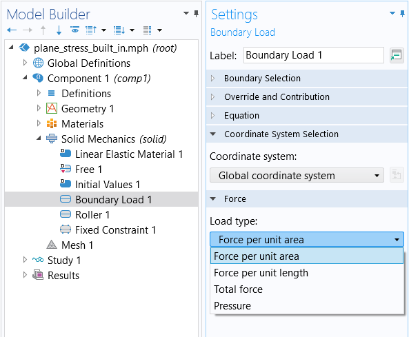
Options for theLoad typesettings for theBoundary Loadboundary condition.

The option for specifying aForce per unit lengthrequires us to specify two vector components:

Compare this with theFlux/Sourceboundary condition of the Coefficient Form PDE:

and we see that we can enter this as:

The option for specifying aPressurerequires us to give a scalar pressure:

where the negative sign on the right-hand side is due to the fact that the normal vector is defined to be directed outward from a boundary of a solid. Note that a negative pressure would then usually be called atension.

We see that we can enter this as

Moving on to constraints, using the built-in interface, we can have aFixed Constraintboundary condition in both displacement variables:

or component-wise:

We can also have aRollerconstraint, which limits movement only in the normal direction of the boundary. This can be written in equation form as:

This is a scalar equation. We can choose to apply this constraint to the first "row" of the equation system and leave the second "row" without a constraint.

To completely constrain a boundary we could add a second constraint

whereis a tangent vector. Note that in 3D, in order to completely constrain a boundary, we would need two tangential constraints using two tangent vectors. Then, you would get various types of constraints by selectively using various combinations of tangential and normal constraints. However, to fully constrain a boundary, you can, of course, more easily use theFixed Constraintcondition described earlier.

A Rectangular Plate with a Circular Hole, Using the Built-In Solid Mechanics Interface

Let us now look at the example from the abovementionedblog post. The example is a simple case of a rectangular steel plate with a circular hole at the center. The rectangle is 2 m wide and 1 m tall, and the hole is centered in the rectangle and has a radius of 0.2 m.

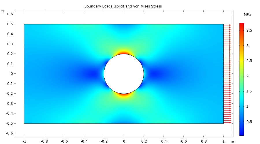
The boundary load and von Mises stress of a rectangular plate with a hole.

An extremely fine mesh setting is used to discretize the model geometry for this example, as shown in the figure below.

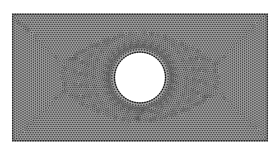
The mesh used in the rectangular plate example. The element type used is second-order triangular Lagrange elements.

In this example model, a tensile load of 1 MPa (1e⁶N/m²) is applied to the right boundary, and the left boundary has a roller constraint. To avoid unwanted vertical motion, the lower-left point is fully constrained. The figures below show the settings for various parts of the interface.

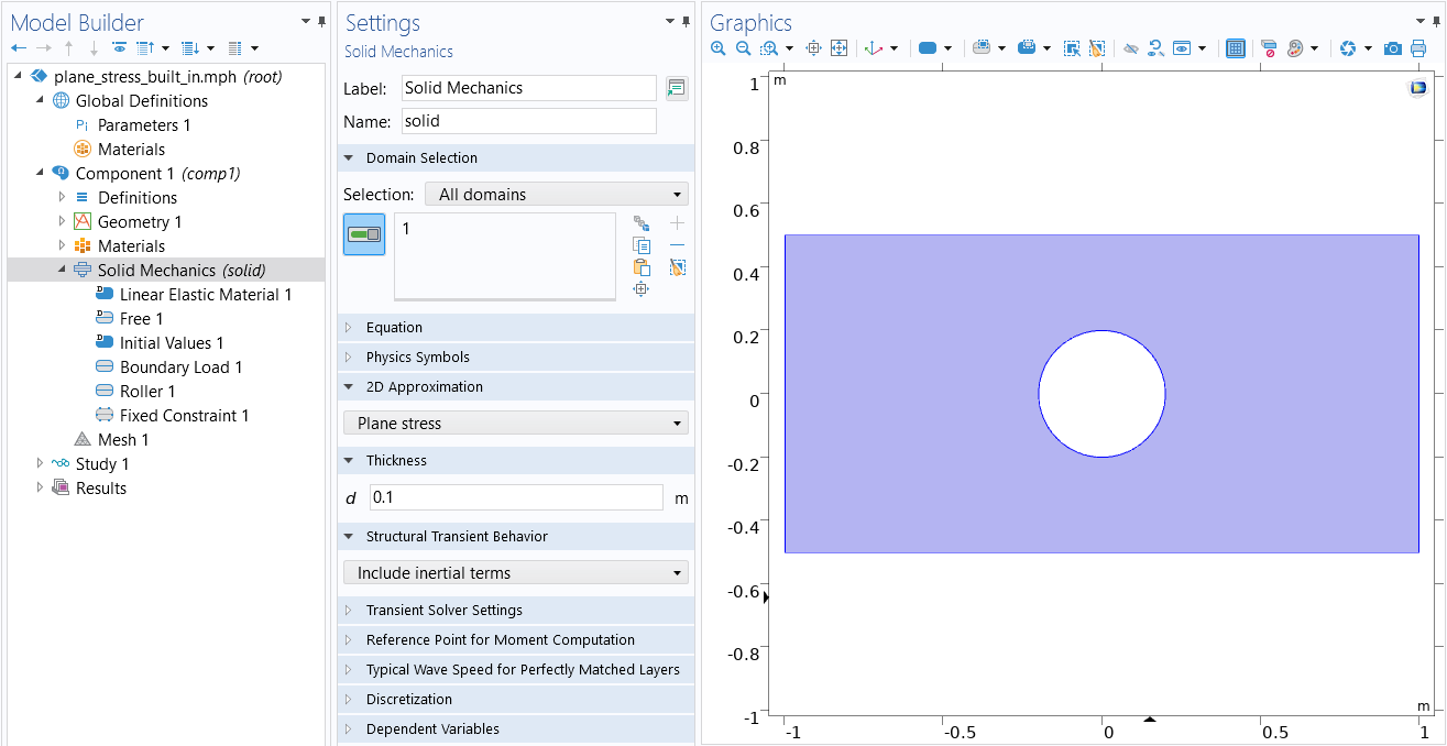The COMSOL Multiphysics UI showing the Model Builder with the Solid Mechanics interface selected, the corresponding Settings window, and the rectangular plate in the Graphics window. TheSolid Mechanics interface with the2D Approximation setting set toPlane Stress. The material used isStructural steel, available from theBuilt-In branch of the material library.

The COMSOL Multiphysics UI showing the Model Builder with the Boundary Load boundary condition selected, the corresponding Settings window with Force per unit area selected as the Load type, and the Graphics window showing the rectangular plate. The boundary condition settings for the tensile load.

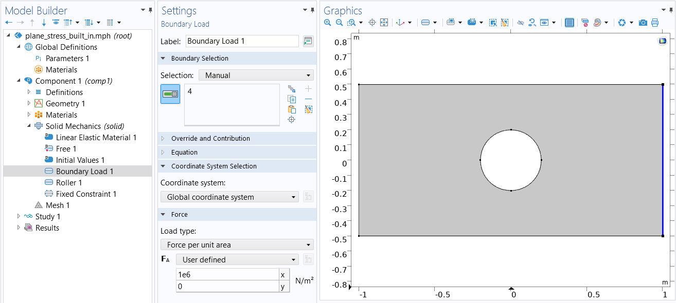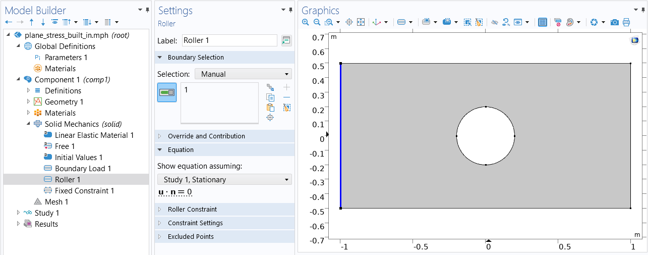The COMSOL Multiphysics UI showing the Model Builder with the Roller constraint selected, the corresponding settings, and the Graphics window showing the rectangular plate. The boundary condition for theRoller constraint.

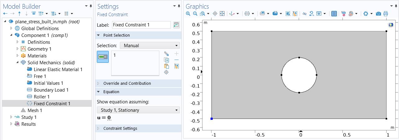The COMSOL Multiphysics UI showing the Model Builder with the Fixed Constraint boundary condition selected, the Fixed Constraint settings, and the Graphics window showing the rectangular plate.
The lower-left point with a fully constrained condition.

The plots below show some of the result quantities that can be evaluated after solving.

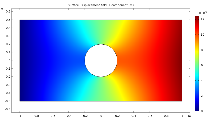
Thex-displacement field, u.

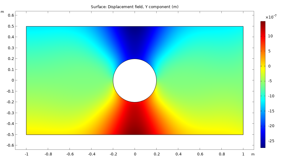
They-displacement field, v.

The shear stresssxy.

A Rectangular Plate with a Circular Hole, Using the Coefficient Form PDE Interface

Now, we will recreate this model using equation-based modeling.

To set up the equations for plane stress, the image below shows theCoefficient Form PDEwith two dependent variables,uandv, for the displacement in thexandydirection, respectively. The defaultDiscretizationsettings forQuadratic Lagrangeshape functions are used. These are sometimes referred to assecond-order isoparametric triangular finite elements.

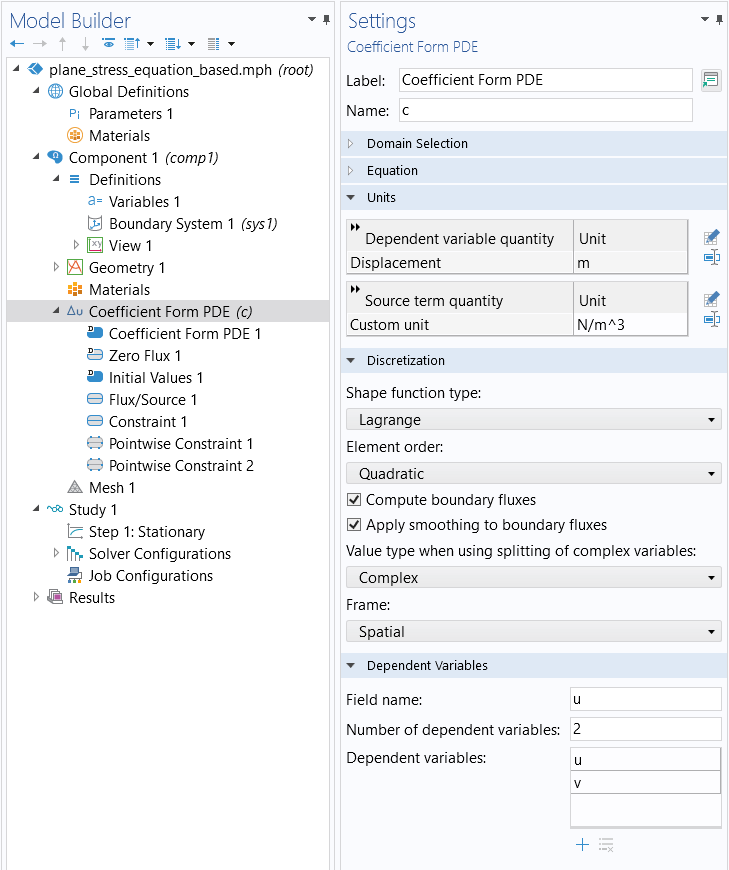
TheCoefficient Form PDEsettings.

In theSettingswindow for theCoefficient Form PDEinterface, change theUnitstoDisplacement (m)for theDependent variable quantityand typeN/m^3for theUnitof theSource term quantity. (There is no built-in option for this unit.)

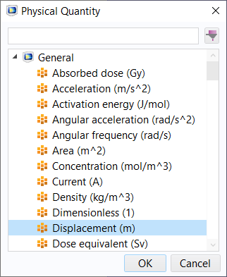
The unit option forDisplacement (m).

Note that you can also determine the dependent variable and unit settings in the Model Wizard, as shown in the figure below.

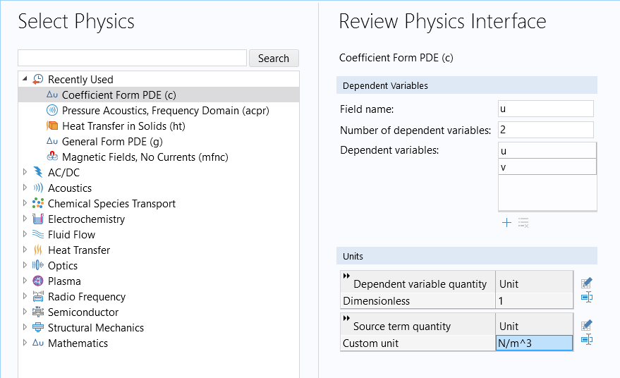
TheSelect Physicswindow in theModel Wizardfor changing the names and number of dependent variables as well as the units.

We will need to define some parameters for the material properties and the thickness.

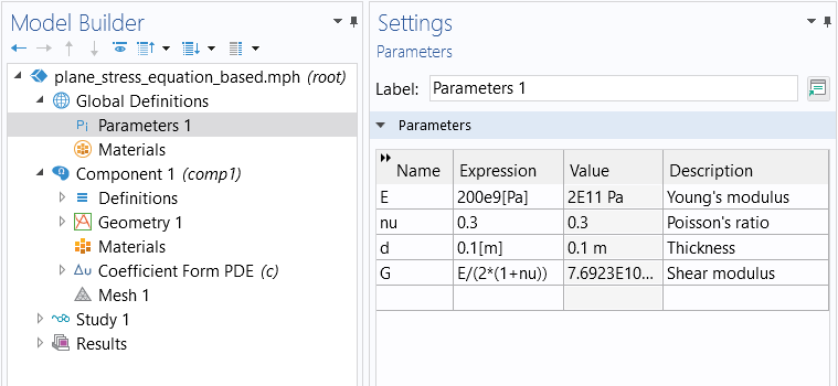
Material parameters for the plane stress example.

The thickness is not needed before or during solving, but to get the right unit when postprocessing the solution.

Recall from earlier that the diffusion coefficient for Navier's equation can be written as:

The figure below shows how to enter the diffusion coefficient components by using theFullandDiagonaloptions.

The Model Builder with the Coefficient Form PDE interface selected and the corresponding Settings window with the Diffusion Coefficient, Source Term, Mass Coefficient, and Damping or Mass Coefficient sections expanded. TheDiffusion Coefficient settings for plane stress.

If you have a body load, with two components

enter these in the fields for theSource Term.

The dynamic coefficientsMass CoefficientandDamping Coefficientare ignored in this model since we are using aStationarystudy.

To specify the boundary load as a tensile load of 1 MPa = 1e⁶N/m³, use theFlux/Sourceboundary condition and have= 1e6 and= 0, as shown in the figure below

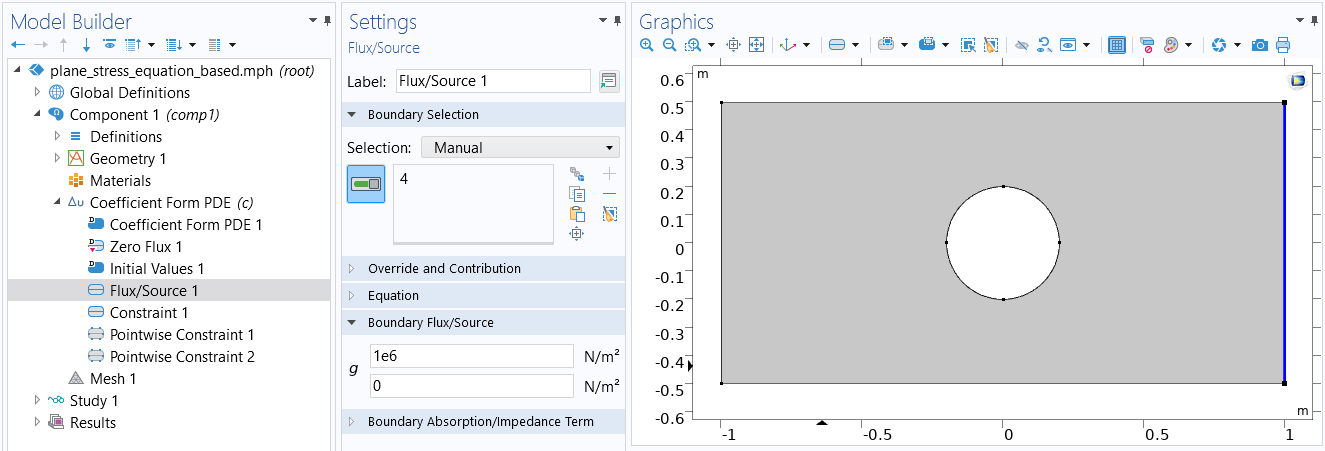
The settings for the tensile load.

In the general case, where the boundary is neither horizontal nor vertical, you can use the variablesnxandnyto define boundary conditions. These variables represent the unit normal vector components, facing outward from a solid domain, on boundaries. For example, in this particular case we would get the same boundary condition by entering= 1e6*nx and= 1e6*ny.

To specify the roller constraint, use theConstraintboundary condition with the constraint

or, written out component-wise,

nx*u+ny*v

You specify this in the fields for the general constraint

Note that since there are two equations, one each for the variablesuandv, we gain access to two constraint fields. However, a roller constraint is a scalar constraint, so we only need to use one of the fields, as shown in the figure below.

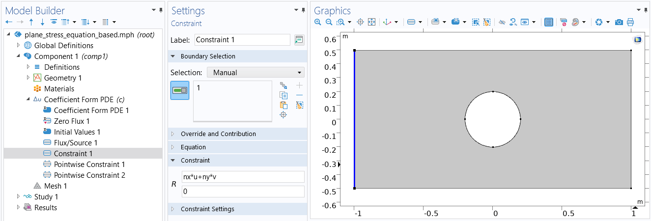The COMSOL Multiphysics UI showing the Model Builder with the Constraint boundary condition selected, the corresponding settings, and the Graphics window showing the rectangular plate. The settings for the roller constraint.

The next step is to fix the displacement of the lower-left point of the rectangle. The built-in interface provides this as one feature node with the combination of both constraints. However, to do so in the equation-based interface we need to use twoPointwise Constraintfeatures, one foruand another forv, as shown in the figures below.

The COMSOL Multiphysics UI showing the Model Builder with the Point Constraint boundary condition selected, the corresponding Settings window, and the Graphics window showing the rectangular plate.The Pointwise Constraintsettings for the displacement variable u.

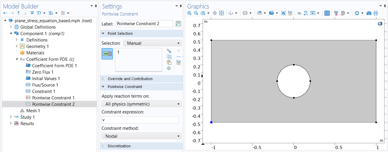The COMSOL Multiphysics UI showing the Model Builder with a second Point Constraint boundary condition selected, the corresponding settings, and the Graphics window showing the rectangular plate. ThePoint Constraint for the displacement variablev.

For convenience, we can now define a set of variables that we would like to visualize or evaluate. The figure below shows the variable settings for the strain and stress tensor components as well as von Mises stress.

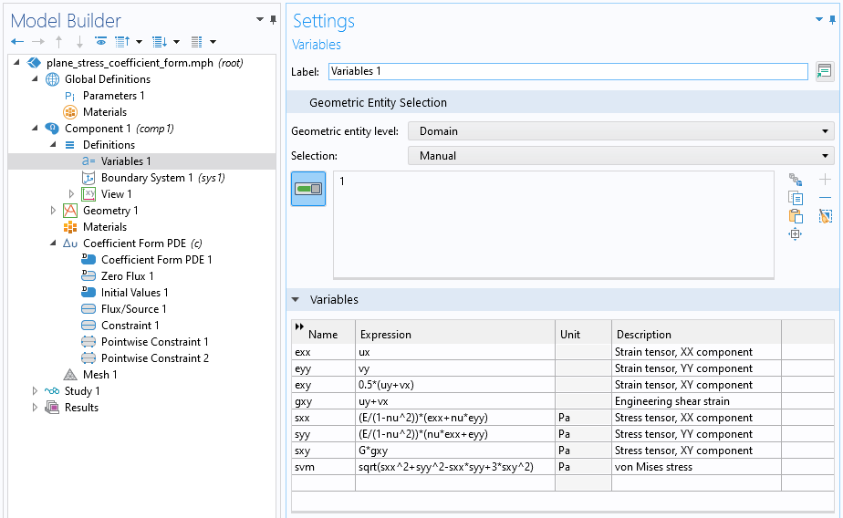
The settings for common structural analysis quantities.

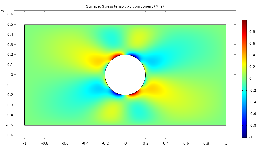
If we now plot these quantities we can see that they are in perfect agreement with the results of the built-in physics interface, as expected if we have entered all the equations correctly. The figure below shows one of the stress tensor components of the equation-based plane stress solution.

The stress tensor componentsxy.

Setting up the plane stress equations using the Coefficient Form PDE requires quite a few steps. In the next couple of parts we will learn about the weak form, which provides a more compact, but also more abstract, way of modeling the same equations.

Further Learning

Although the model used as the example throughout this article is available for download, we encourage you to first build the model yourself, completely from scratch, by following the guidance provided throughout this article. Thereafter, you can open and explore the model files for both the version of the model built using theCoefficient Form PDEinterface, as well as the version built using the software's predefined physics interface. This will reinforce learning how to set up equation systems from scratch.