学习中心

Integrating Along Streamlines and Extracting Particle Statistics

---

Given a computed steady-state flow field, it is often desirable to compute quantities such as the residence time distribution function of the fluid within the domain, as well as other statistical data related to the distribution of times that it takes the fluid to pass through the domain. This article addresses such situations.

Modeling Notes

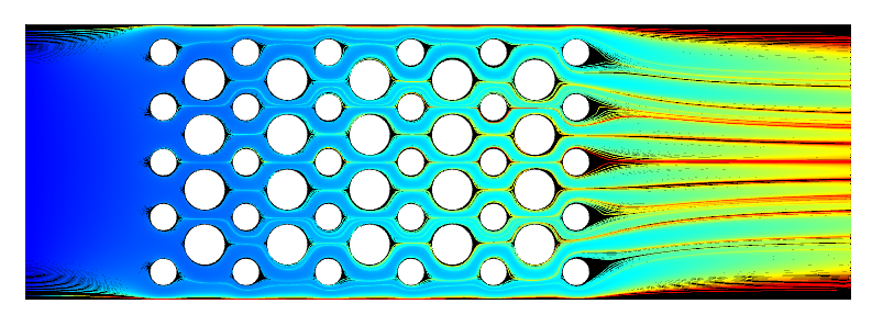
This example is presented in the context of a steady-state laminar flow field, representing the flow through a small device, as visualized in the image below. A fluid inlet is defined on one side of the domain, with a parabolic velocity profile, and a uniform pressure outlet defined on the other side. TheLaminar Flowinterface is used, and the model is solved as a stationary problem.

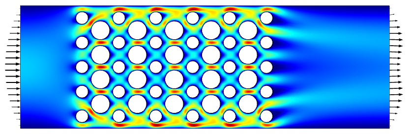
The computed steady-state laminar flow field through a device.

Beginning with a model that has a steady-state flow solution, add aParticle Tracing for Fluid Flowinterface. Within the settings, specify to use aMasslessformulation for the particles, and specify to store the particle status data. Within theParticle Properties, specify the particle velocity to be the flow field components,u,v, which is equivalent to defining a computational particle that traces streamlines.

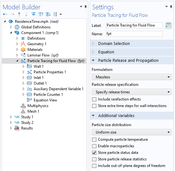
Settings for theParticle Tracing for Fluid Flowinterface. Massless formulation is used. Particle status data is stored.

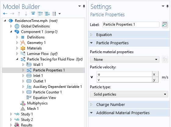
Particle Propertiessettings. The particle velocity is the fluid velocity.

AnInletcondition is defined at the same boundary as the fluid inlet, and particles are released at time zero. The distribution of particles along this boundary is set to be proportional to the fluid velocity, since there are more particles of fluid passing through the domain where the inlet velocity is higher.

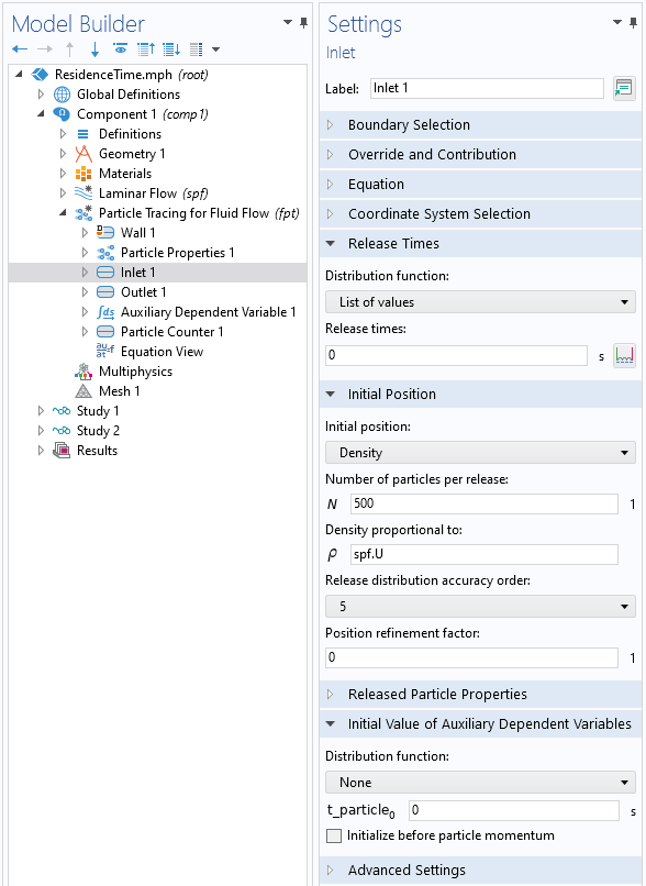
Settings for the particleInletcondition.

As the computational particle moves along this streamline, an additionalAuxiliary Dependent Variableis used to monitor the time for each particle as it moves through the domain and gets to the outlet boundary. As shown in the screenshot below, theAuxiliary Dependent Variabledefinest_particle, with units of time. By integrating the source term,R = 1, with respect to time, this variable will track the time as the particle is traced through the domain. Once the particle reaches the outlet, this variable is frozen to the exit time. AParticle Counterfeature is also applied at the boundary to monitor statistics of the particles as they leave the modeling domain.

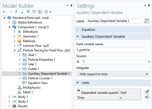
AnAuxiliary Dependent Variableis defined on each particle.

A separate study is used to compute the particle paths and uses the results from the first study. The output times specify how long to trace the particles, and how many output time steps are saved. It is not known ahead of time how long it will take for the particles to traverse the modeling domain, so the maximum time has to be studied. The intermediate output time steps, between the start and end time, only need to be saved if a visualization of the residence time is desired.

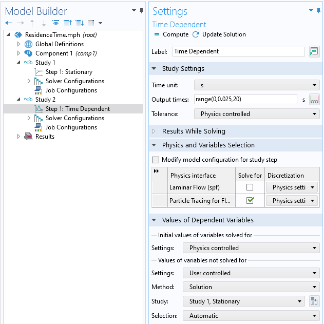
Settings for the second study, which computes the particle paths.

Results Extraction

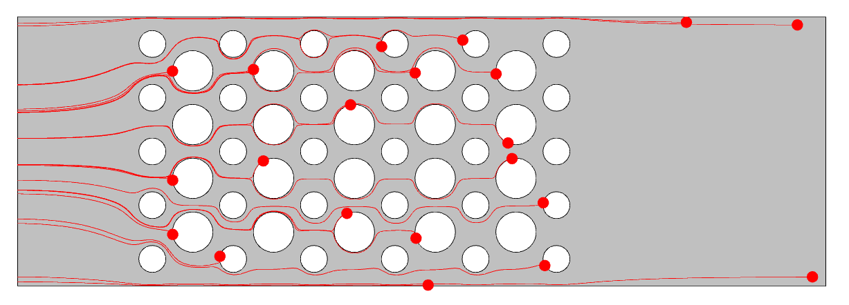
To visualize the residence time, add aParticle Trajectoriesplot and color it using the particle time variable. This plot will look more smooth as more output time steps are saved. If this plot is not desired, save only the start and end times as the output times.

Visualization of streamlines, colored by the residence time variable.

It is also possible to plot those particles that have not yet left the modeling domain. These particles follow streamlines that pass very close to a wall, where the velocity approaches zero, leading to a trapping effect. This can be reduced with mesh refinement near the walls, although this is not always desirable due to the increased computational cost for solving the fluid flow problem. In reality, there will be some diffusion as well, but this is ignored when using the massless particle tracing formulation. One approach is to filter these remaining particles out of the results, and theParticle Counterfeature creates a logical variable, defined on each particle,fpt.pcnt1.rL, which is true if the particle reaches the outlet.

Visualization of those particles left within the computational domain at the end of the simulation time.

To plot the residence time distribution function, use theHistogramplot type, and plot either theAuxiliary Dependent Variableof the particle time or theParticle Statusstop time. Use theSum of valuesnormalization of the output. To plot the cumulative distribution, use the same kind ofHistogramplot, withPeaknormalization, with theCumulativeoption enabled. Plot for the last time stored. TheFiltersubnode is added to theHistogramplots to filter on theParticle Counterlogical expression.

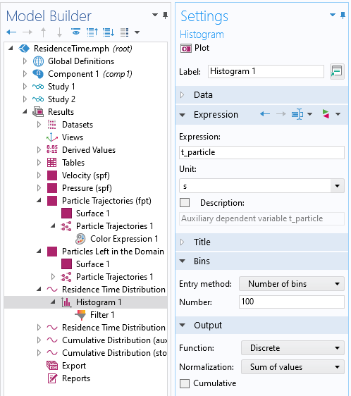
Histogramplot settings for residence time distribution function.

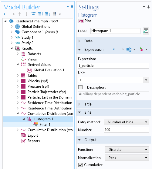
Histogramplot settings for cumulative distribution function.

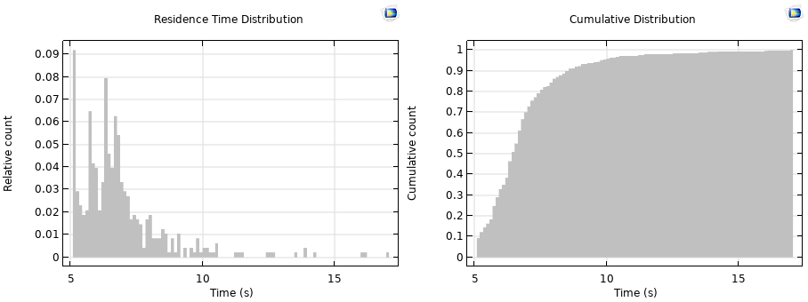
Plots of residence time distribution (left) and cumulative distribution (right).

To compute the mean residence time, use nonlocal coupling operators viaResults>Derived Values>Global Evaluation. The expressionfpt.fptop1(fpt.pcnt1.rL*t_particle)/fpt.fptop1(fpt.pcnt1.rL)will average the residence time variable over all particles that have left the modeling domain. Here,fpt.fptop1is a predefined operator to compute a sum over all particles. The same operator can be used to compute the variance, as well as construct other metrics.

The supplementary model file with this example is available below.