Viewing and Accessing the Equations and Variables for Physics Feature Nodes
In COMSOL Multiphysics®, you can see the underlying governing equations for the physics in a model, as well as the definitions of the variables. This enables you to:
- See how the variables are calculated by the software
- See the names of variables and the quantities each one defines
- Access and use the variables when formulating expressions
- Edit any variables and equation contributions defined and used internally by the software
- More easily search and find variables defined by each physics interface and physics feature node
- Define custom multiphysics couplings between physics interfaces
In this article, you will learn how to both view and access the equations and variables for physics feature nodes. We will also demonstrate how to perform all of the items listed above using an example toward the end of this article.
Seeing the Equations
You can see the equation for any physics node in your model by selecting the respective node and in theSettingswindow, expanding theEquationsection.
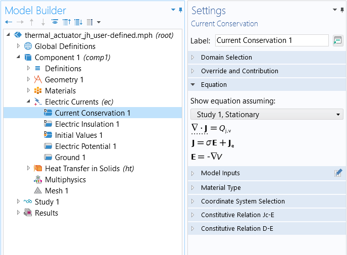
TheSettingswindow for theCurrent Conservationnode, wherein theEquationsection has been expanded.
In theEquationsection, the mathematical equations applicable to the node, and the selected study type, are displayed. The terms being contributed to the equation by the node are also highlighted with a dotted line displayed under the respective part of the equation (as seen in the above screenshot), except for the parent physics interface node (shown below).
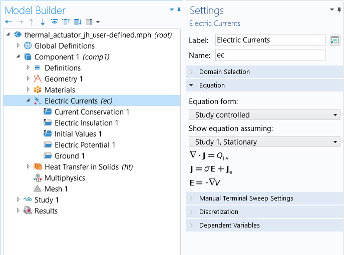
TheSettingswindow for theElectric Currentsphysics interface, wherein theEquationsection has been expanded.
Accessing the Equations and Variables
Equation View
You can access the equations and variables used internally by COMSOL Multiphysics®by enabling theEquation Viewnodes to display in the model tree. Through theModel Buildertoolbar, you can open the menu for showing more options, and then select the check box next toEquation Viewand clickOK.
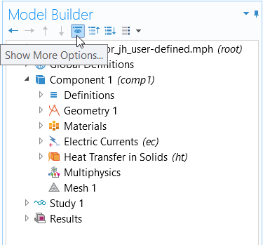
TheShow More Optionsdialog box accessed through theModel Buildertoolbar.
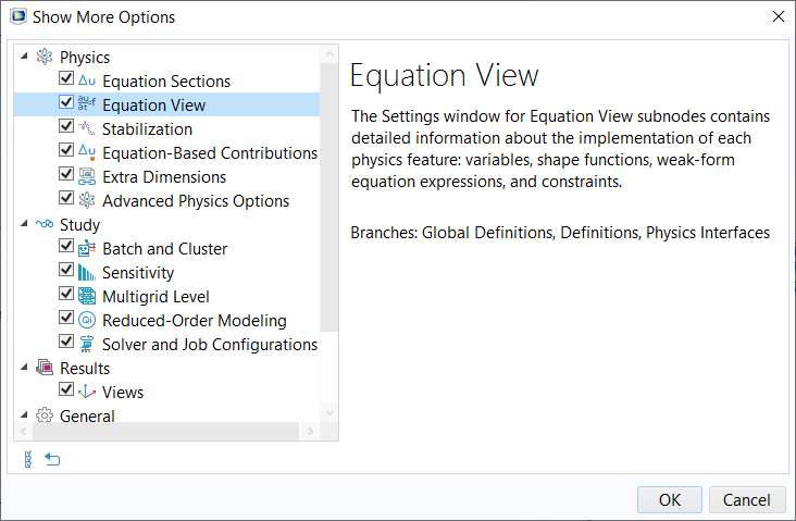
Enable displaying theEquation Viewnodes for all the physics feature nodes in your model tree by selecting the respective check box.
Once enabled, there will be anEquation Viewnode underneath each physics node that contains a list of all internally defined variables for the respective node. In the settings, you can see the variable names, expressions, units, and descriptions, among other details. All the variables and equation contributions defined by each node in a physics interface become visible and editable (such as to couple physics). You can easily search this information to find the variables you are looking for using theFind tool.
 A screenshot of the Equation View Settings window with an expanded table of variables
TheEquation View for theCurrent Conservation node, wherein the table listing the variables has been expanded.
The Report Node
You can also access the equations and variables used for the physics through using theReport Generator. This tool enables you to document all the details of your entire model. You can generate a report that displays within the software and includes this information by completing the following steps:
- Select and right-click theReportnode
- Choose to generate aComplete Report
- Select the option in the settings toPreview Allof the report
- A preview of the report will appear in a new tab in theGraphicswindow
- Navigate to the physics interface or physics feature node which you want to see the equations and variables for
Generating a complete report for a model and searching for the equations and variables for a specific physics feature node are demonstrated.
The reportPreviewtab in theGraphicswindow provides you with a convenient, at-a-glance view of all the equations and variables for the physics nodes. The information is displayed all at once without needing to switch between selecting different nodes. In addition, the expanded table formatting used for the variables' sections enables you to easily see all the settings and details for each.
 A screenshot of part of a report from a model that includes the Electric Currents interface, with columns for Name, Expression, Unit, Description, Selection, and Details.
An excerpt of a report from a model including theElectric Currents interface.
In COMSOL Multiphysics®, the ability to see and access equations and variables for the physics feature nodes included in your model are necessary in order to make changes, such as for implementing manual, custom multiphysics couplings. Below, we show a brief demonstration of this, the full process for which is detailed in anotherLearning Center article.
User-Defined Multiphysics Couplings
The ability to define arbitrary, and user-defined, couplings between existing physics interfaces is one of the core capabilities of COMSOL Multiphysics®. Although there are manymultiphysics couplings already built into the software, in some cases, you may want or need to create your own. Here, it is briefly shown how an existing coupling is introduced, and how to implement the same coupling manually using the aforementioned features. TheThermal Actuator tutorial modelis used as our example. Further discussion of this topic, along with a comprehensive introduction, is provided in an articleDefining Multiphysics Models Manually with User-Defined Couplings.
An Existing Multiphysics Coupling: Joule Heating
One of the more common examples of a multiphysics coupling is Joule heating, where the flow of electrical current through a conductive material leads to heat losses, which lead to a rise in temperature. In short, to solve for Joule heating, one must solve for both the electric currents as well as the heat transfer governing equations. The stationary (time-invariant) form of the partial differential equation for electric currents is:
whereis the current,
is the electric field,
is the electric conductivity, and
is the electric potential.
For heat transfer, the governing equation is:
whereis the thermal conductivity and
is the temperature field.
The Joule heating effect introduces a heat load of the form:
The above coupling is automatically included via theElectromagnetic Heatingmultiphysics coupling feature, as shown in the screenshot below.
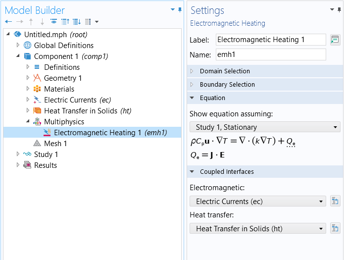
The predefined multiphysics coupling for Joule heating.
Simply by adding this feature and applying it to all relevant domains, the above multiphysics coupling will be included in the model. It is also important to note that this feature will automatically account for any nonlinear material properties, such as, for example, thermal and electrical conductivities that are temperature dependent. To learn how to define material properties that are dependent upon variables being solved for, you can watch a tutorial video onusing functions to define material properties.
Manually Implementing a Multiphysics Coupling: Joule Heating
To manually implement this same multiphysics coupling, you will need to be aware of the full equation that you want to implement, as well as how variables are implemented within the COMSOL Multiphysics®architecture. First, we expand the full equation that we want to implement, the source term in theHeat Transfergoverning equation:
wherehere is an isotropic (scalar) value.
In the most general case, it can be an anisotropic tensor:
Next, we need to know what all of these variables are called, internal to the COMSOL Multiphysics®architecture. As aforementioned, this can be done either through enablingEquation Viewor using theReport Generator. The screenshot below shows the variable name, expression, unit, and description for the components of the electric conductivity tensor, as well as the isotropic value. We can use theFindtool to search for these quantities and locate the respective variables and expressions that define them. If we are only interested in searching within the report preview, we can select the respective tab for it in theGraphicswindow and use the keyboard shortcut Ctrl+F to search locally within the generated report preview text.
 A screenshot of the Settings window for the Equation View node, with the Study and Variables sections expanded.
The equation view, showing the components of the electric conductivity tensor and its isotropic value.
An excerpt from this report is included below, and shows the names of the electric field components and how they are defined. The partial derivatives of
V(the field variable representing the electric potential) are given by the notation
Vx,
Vy,
Vz, the partial derivatives in the
x-,
y-, and
zdirections, respectively.
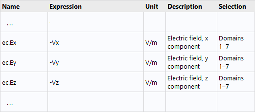
An excerpt of a report from a model including theElectric Currentsinterface.
Now that all internal variable names are known, all that remains is to manually add the heat source term to theHeat Transfer in Solidsinterface. The expression for the source term can be written several different ways using the variables shown above. However, if we assume isotropic electric conductivity, one convenient way to write it is:
ec.sigma_iso*(ec.Ex^2+ec.Ey^2+ec.Ez^2)
The expression can now be added as a domainHeat Sourceterm within theHeat Transfer in Solidsinterface, as shown in the screenshot below. Note that once you add this coupling manually, you should remove the built-in coupling from theMultiphysicsbranch, which was shown earlier. Again, keep in mind that any nonlinearities present in the materials will be automatically incorporated into this definition.
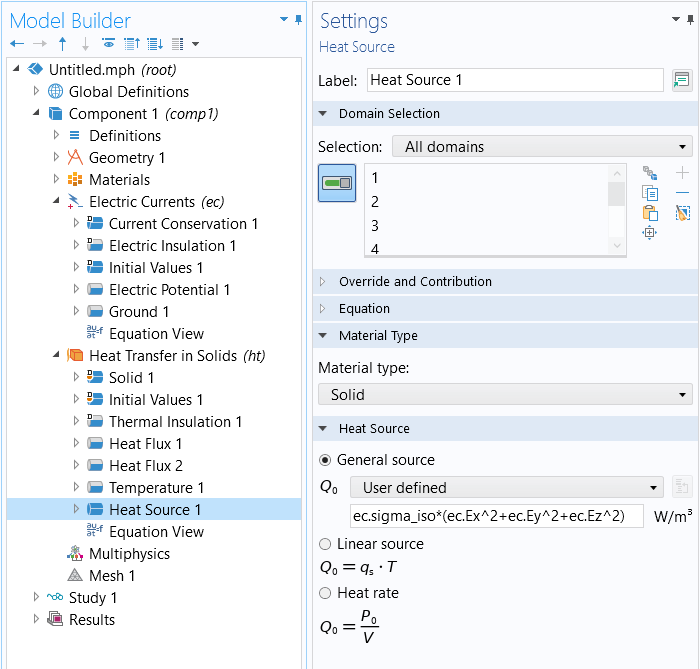
A manual implementation of the Joule heating multiphysics coupling.
Further Learning
Regardless of the multiphysics couplings that you will want to implement manually, the approach will be similar to what has been briefly described above anddiscussed in detail separately. The overall approach is the same if implementing couplings on domains or as boundary conditions. Note that such couplings will almost always result in a nonlinear problem. If you are not using the existing physics interfaces in the software, you will need to manually create and define yourself all of the intermediate variables and nonlinear material relationships via variables and functions features underneath theDefinitionsnode. For this and other reasons, we highly recommend taking advantage of the software'spredefined multiphysics interfacesorpredefined multiphysics couplingswhenever possible. Some examples of models that demonstrate manual couplings include:
- Transport and Adsorption
- Vacuum Drying
- Tubular Reactor with Jacket
- Chemical Etching
- The Shallow Water Equations
If you are solving such models as a stationary (time-invariant) problem, see:Improving Convergence of Nonlinear Stationary Models. Or, if solving in the time domain, see:Controlling the Time Dependent solver timesteps.
请提交与此页面相关的反馈,或点击此处联系技术支持。
