Two-Phase Flow Modeling Guidelines
When modeling fluid flow in COMSOL Multiphysics®using any of the physics interfaces that fall under theTwo-Phase Flow, Level SetorTwo-Phase Flow, Phase Fieldapplication areas, there are several guidelines you can follow to ensure that your model converges and does so both in a reasonable time and to a reasonable result. Here, you will find guidance for solving these types of fluid flow problems.
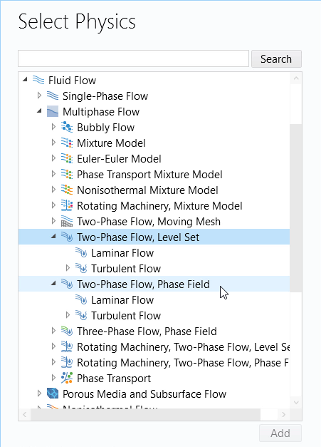
TheTwo-Phase Flow, Level SetandTwo-Phase Flow, Phase Fieldbranches of physics interfaces in theSelect Physicswindow.
Background
Fluid flow is governed by the Navier–Stokes equations, which solve for fluid velocity and pressure fields everywhere within the modeling domain. The fluid properties (viscosity and density) are either constant or vary relatively smoothly in space as a function of temperature, pressure, shear rate, etc. However, if we want to model two immiscible fluids, then the fluid properties will vary significantly across the interface between the two fluids. The surface tension effects can become important, as well as the effect of contact angles at wetted walls.
To model this in COMSOL Multiphysics®, we can use either the level set or phase field method. Both of these methods introduce an additional scalar field (the level set or phase field function) to the modeling domain. These scalar fields vary smoothly between -1 and +1 everywhere and are used to define the fluid viscosity and density in the governing Navier–Stokes equations. The transition (where the fields vary from 0 to 1 for the level set implementation and -1 to +1 for phase field) is quite abrupt in space, thus giving a good resolution of the two phases. The governing equations for the level set and phase field methods are a type of convection–diffusion equation, with the advective velocity coming from the Navier–Stokes equations. Such equations are, however, quite numerically challenging to solve due to the combination of the significant advective term, abrupt transition in the field, and strong coupling to the Navier–Stokes equations.
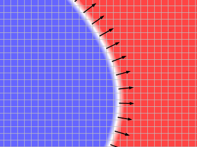 A visualization of the level set function defining the interface between two fluids, shown in red and blue, with black arrows showing the advected boundary.
Options and General Guidelines for Modeling Two-Phase Flow
If you want to model two-phase flow that does not involve any topology changes (that is, no droplet breakup, free surface formation, etc.), and if the free surface does not undergo significant shape changes, you may be able to use theLaminar Two Phase Flow, Moving Meshphysics interface. This formulation, if it can be used, will require less computational resources. Regardless of the physics interface used, there are general guidelines that can be used when modeling this type of flow. These are listed below and organized by the modeling workflow step.
Geometry
If at all possible, begin your modeling in 2D or 2D axisymmetry. Such models will be significantly faster to solve than 3D models and serve as a useful test for trying out different model settings that will be applicable for 3D models.
If reasonable, avoid sharp edges and corners at any boundaries where you expect the interface between the two fluids to traverse. Introduce a fillet in the geometry so that there is a smooth transition between boundaries.
Physics
All fluid inlets should be in regions where there is a single phase entering the modeling domain, and the phase entering at that inlet should match the initial phase inside the adjacent domain. You may need to alter the geometry slightly to achieve this.
For both the level set and phase field approaches, there is aTwo-Phase Flow, Level SetandTwo-Phase Flow, Phase Fieldfeature under theMultiphysicsnode. Make sure to choose the appropriate materials from the drop-down lists forFluid 1andFluid 2in the settings.
Within theLaminar Flowphysics interface, make sure to use the incompressible formulation. You should also make sure that all specified velocities or pressures at inlets ramp smoothly up from consistent initial conditions, which is described in more detailhere. For models involving gravity, make sure to enable theInclude gravityoption under the settings for theLaminar Flowphysics interface, instead of using aVolume Forcecondition. This is so that the hydrostatic pressure is automatically taken into account under theInitial Valuesnode and under other pressure conditions.
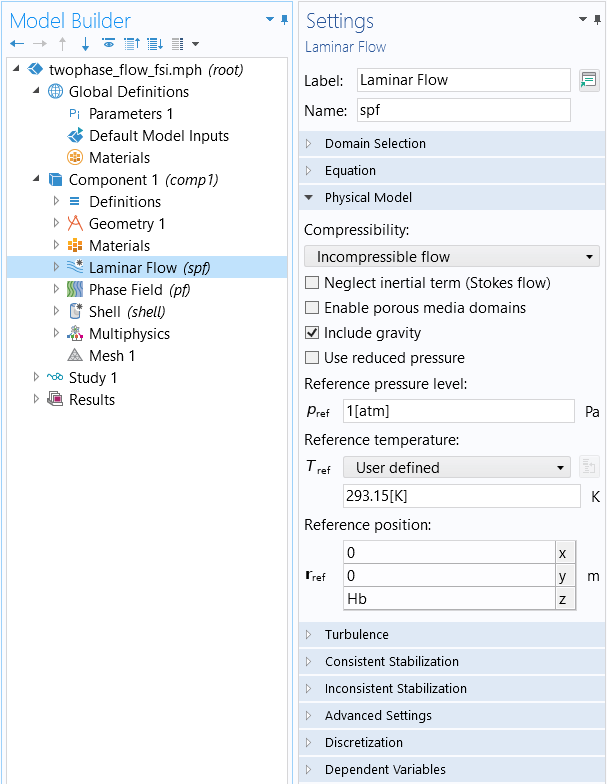 A screenshot of the Settings window for the Laminar Flow interface, with the Physical Model section expanded and showing the recommended settings.
If modeling bubbles with surface tension, make sure to define the additional initial pressure inside of the bubble that balances the surface tension. A reasonable value for this initial pressure can be computed from the Young–Laplace equation.
When using either theLevel SetorPhase Fieldphysics interfaces, there is aLevel Set ModelorPhase Field Modelfeature, which is used to define theParameter controlling interface thickness. If this value is too small, it can lead to numerical instabilities. If it is too large, the interface movement is not captured correctly. The parameter controlling the interface thickness is set proportional to the maximum element size:hmax.
 A screenshot of the settings for the Phase Field Model feature, with the Phase Field Parameters section expanded.
When using thePhase Fieldphysics interface, thePhase Field Modelfeature also defines theMobility tuning parameter. Again, too small a value leads to numerical instabilities, and too large a value will not capture the interface movement correctly. A good initial estimate for theMobility tuning parameteris:
2*umax/(3*sqrt(2)*sigma)*(hmax/epsilon)
whereumaxis the expected maximum velocity magnitude;sigmais the surface tension coefficient;hmaxis the value of the parameter controlling the maximum element size; andepsilonis the value of theParameter controlling interface thickness.
When using theLevel Setphysics interface, theLevel Set Modelfeature also defines theReinitialization parameter. If the reinitialization parameter is too small, it can lead to numerical instabilities. On the other hand, if it is too big, then the interface movement is not captured correctly. A good estimate for the reinitialization parameter is the maximum expected velocity magnitude.
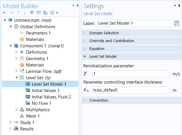 A screenshot of the settings for the Level Set Model feature, with the Reinitialization parameter and Parameter controlling interface thickness options shown.
When using the level set approach, there is aWetted Wallmultiphysics coupling boundary feature, and when using the phase field approach, there is aWetted Wallnode that specifies aContact angle. This contact angle should be in agreement with the actual initial angle of the two phases, as defined by the geometry and thePhase Field/Level Set>Initial Valuesfeature. If the contact angle as defined by the initial values is different, then the specifiedContact angleshould be ramped up in a way similar to the velocity ramping (see:Solving time dependent CFD simulations).
In the settings for theLaminar Flow,Level Set, andPhase Fieldphysics interfaces, there is aDiscretizationsection where you can change the element order. The default discretization isP1+P1for theLaminar Flowphysics interface, andLinearfor theLevel SetandPhase Fieldphysics interfaces. Higher-order discretization will be significantly more computationally intensive and is not usually recommended. Instead, you can refine the mesh.
Mesh
The mesh should have roughly equal size throughout the modeling domain, and the mesh elements should beasisotropicas possible; that is, the elements should not beoverlystretched or compressed in one direction. The mesh size must be small enough to give a good resolution of the fluid interface between phases. A good rule of thumb is to begin with a global element size that is one-tenth of the smallest expected droplet size, and to refine the mesh from there.
Define a parameterhmaxthat is used within theMesh>Sizenode's settings to define theMaximum element sizein all domains. Once you have arrived at a converged solution on a particular mesh, repeat the analysis with a smaller mesh size. Once the solution does not change significantly with mesh refinement, the solution can be converged with respect to the mesh.
If it is known that one subdomain of the entire modeling domain will only ever contain the same fluid phase, then a coarser mesh can be used in that subdomain.
There is not a significant difference between structured and unstructured meshes for modeling these types of problems.
Study
The study always consists of two steps. First, aPhase initializationstep initializes the level set or phase field variable such that it is smoothly varying everywhere. Next, aTime Dependentstep simultaneously solves the Navier–Stokes equations and the level set or phase field equation.
Within theTime Dependentstudy step settings, there is aTolerancefield that defaults toPhysics controlled. This can be changed toUser controlled, and tighter solver relative tolerances should be investigated to confirm that the solution is converged with respect to relative tolerance. That is, once a solution is computed, repeat the solution with a finer solver tolerance. Once the solution does not change significantly with solver tolerance as well as mesh refinement, the solution can be considered converged. You should not study finer solver tolerances before addressing all of the other above guidelines.
 A screenshot of the Settings window for the Time Dependent study, with the Study Settings section expanded and the Tolerance set to User controlled.
请提交与此页面相关的反馈,或点击此处联系技术支持。