学习中心

Coupling Physics Between Model Components for Multiphysics Models

---

In COMSOL Multiphysics^®, if you are simulating several components in a system, or a complete model that has submodels, you can manually couple the physics in different model components when needed. This type of coupling is one example of the manual approach with user-defined couplings. In this article, we discuss how to perform this specific type of multiphysics coupling and direct you to resources that provide further details on how to accomplish this for different scenarios.

Background

In certain cases where it is either motivated to do so or necessary (which we will address later in the article), you may need to model several components in a system and then couple the models to simulate a part of the system or the whole system. Although COMSOL Multiphysics^® is not a traditional systems modeling tool, you can model several components and couple them into a systems model. This coupling can be done using variables and derived variables. In the software, each physics interface defines the equations, dependent variables, and a set of derived variables for the respective physics being simulated. For example, in the figure below, an ideal continuous stirred tank reactor (CSTR) modeled in 0D is coupled with a 2D model of a dialysis membrane cell using derived variables. The model represents a real system where a salt in the dialysate is removed over time by continuously pumping the dialysate over the dialysis cell. Mapping from one component to another can also be done for components in different space dimensions with completely different geometries through the use of nonlocal couplings (there will be more on this later).

Schematic (left) and the coupling between the components (right) of the membrane dialysis with a two-layered membrane tutorial model. The model contains two model components, including a 2D membrane unit (component 1) and 0D CSTR (component 2). The model components are coupled through the flow from the membrane unit being defined as the feed into the CSTR and the flow out from the CSTR being defined as the inlet condition to the membrane unit.

Simulations that demonstrate the use of these types of couplings among multiple model components are detailed farther below.

Examples of Multicomponent Couplings

Models that involve multiple components and use couplings between them include system models, if you are employing a submodeling technique and are mapping the results from a global model to a submodel, linking between two submodels, or otherwise need to split your analysis among multiple components for efficiency to save computational time and resources. Some multiphysics examples and others that demonstrate this and are available in the Application Libraries include:

• In the Thermal Modeling of a Cylindrical Lithium-Ion Battery in 3D tutorial model, a 1D model component is used to model the battery cell chemistry and a 3D model component is used to model the temperature in the battery. The two components are coupled by the generated heat source and average temperature.
• In the Noise Radiation by a Compound Gear Train tutorial model, the multibody dynamics and acoustics analyses are performed in separate model components, so the multibody setup is not affected. A General Extrusion nonlocal coupling operator is used to map the acceleration between the model geometries.
• In the Ultrasonic Flowmeter with Piezoelectric Transducers tutorial model, the entire model is split into three submodels, as different parts of the model require the use of different discretization methods as well as time-dependent solvers. An Identity Mapping nonlocal coupling operator is used to map the results between the submodels and couple them.
• In the Energy-Based Thermal Fatigue Prediction in a Ball Grid Array tutorial model, a full model of the microelectronic component is analyzed with a coarse mesh to generally find any critical parts of the design. A second submodel of the critical region is then made to be studied in detail. The physics from the component containing the global model are coupled with the component containing the submodel through nonlocal couplings and the Prescribed Displacement and Temperature boundary conditions.
• In the Submodel in a Wheel Rim tutorial model, the entire wheel rim is modeled in one model component to analyze the stiffness of the structure. A second model component is then used to create a model of the region around one of the spokes to analyze the stress concentration using a fine mesh. The submodel is solved using the displacements from the full global model as boundary conditions for the local submodel.

Regardless of how the coupling is carried out and for what reasons, the variables or solution data from one model component is made accessible and available for use in another model component. A general framework for how to perform such couplings between model components is outlined below.

Setting Up Multicomponent Couplings

There are a variety of ways that we can couple the physics between model components. Although there is no specific set of steps that need to be followed, we have outlined a plan you can use to conduct such couplings. It can generally be done through the use of nonlocal couplings and coupling operators and/or derived variables, which we introduce and present the steps for here.

Nonlocal Couplings

Nonlocal couplings create couplings between different model components, or different parts of a model component, and are defined through the use of a coupling operator. They create these couplings by mapping variables from a source model geometry (domains, boundaries, etc.) in one component to a destination model geometry in another component (or another geometric entity in the same component).

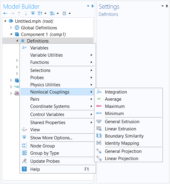
Menu for the nonlocal couplings that you can add to a model component, accessed through the Definitions node in the model tree.

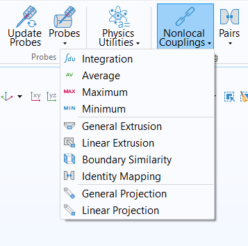
The button for adding Nonlocal Couplings, which is accessed through the Definitions ribbon tab.

The way this mapping occurs is through the coupling operator evaluating an expression that is supplied as the argument in the source model geometry and then defining the result in the destination model geometry. This is explained in detail in our blog posts on accessing nonlocal variables with Linear Extrusion operators and mapping variables with General Extrusion operators. A general procedure for creating couplings through these means would be as follows:

1. Add the physics interfaces under their respective model components
2. Define the physics settings for each physics interface
3. Define the multiphysics couplings
   a. Add a nonlocal coupling to the source component
   b. Define the coupling operator
   c. Incorporate the coupling operator with the appropriate argument in the destination component
   d. Compute the solution to the model equations
   e. Check the results
4. Repeat Step 3 for each subsequent multiphysics coupling or coupling between components

The logic behind dividing defining the physics into two parts (first defining each individual physics interface and then defining the couplings) in the procedure is explained in the Learning Center article on the manual approach with user-defined couplings. Namely, it enables you to search the dependent variables and derived variables as well as access the variable names when formulating expressions for any equation contributions. It should also be noted that in the abovementioned procedure, the nonlocal coupling must be added under the component containing the variables you want to access in other components. Then, within the settings or definitions of the other model components, you enter the coupling operator using the correct syntax. From there, the appropriate expression for the argument of the coupling operator must be used in order to have the desired quantity defined in the component locally.

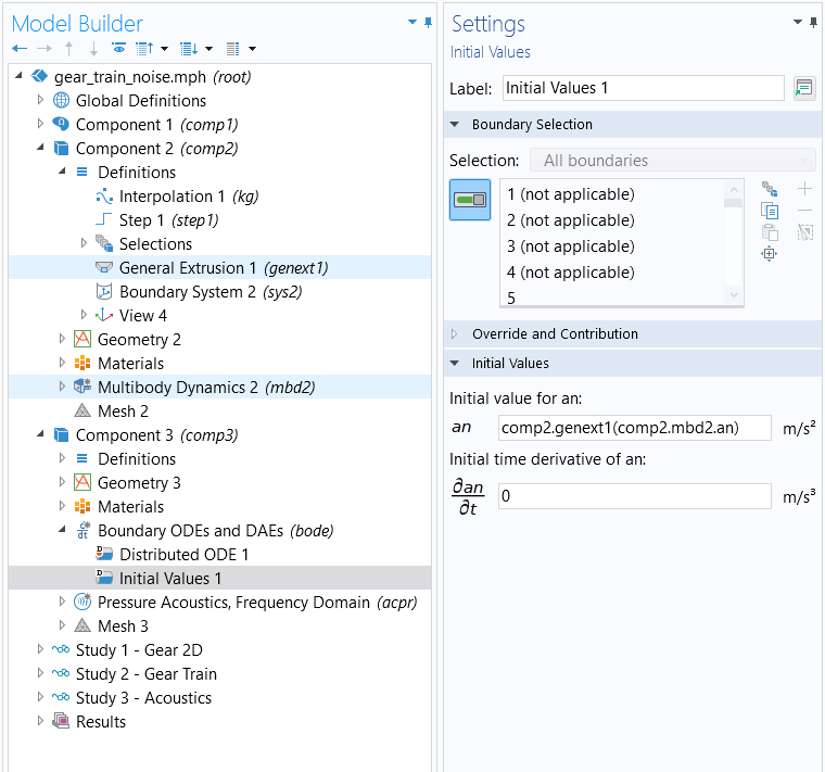
The settings for the Compound Gear Train Noise radiation tutorial model. A General Extrusion operator is defined in the second component and used in the third component under the Initial Values node to map the acceleration between the model geometries.

Derived Variables

Apart from using nonlocal couplings, in specific cases you can administer physics couplings between components by including the variables from one model component directly in the settings and definitions of another model component. This can be accomplished in the case where the source variable (variable A in component 1, for example) is defined with a global selection (seen under Equation View nodes in the Selection column of the table with variables). Being "global" and not bound to a specific domain, edge, or point, the variable can be evaluated in any other interface.

If this is not the case, the variable is defined on a specific geometry selection (domain, edge, point) locally in the component and is not available in another component and a coupling feature is needed.

Interfaces in 0D model components define variables with Global selection. In the Reaction Engineering and Chemistry interfaces, variables are usually defined with global selection. The purpose of these interfaces is to produce variables to be used in other interfaces.

Some examples of this coupling are included here:

Model	Components	Coupling Between Components
Time-Dependent Model of Membrane Dialysis	• 2D membrane     unit • 0D continuous     stirred tank     reactor model	1. Flow out from the membrane feeds into the CSTR      • Concentration      • Volumetric feed rate 2. Flow out from the CSTR is defined as the inlet     condition for the membrane unit      • Concentration
Protein Adsorption	• 0D reactor     system • 3D model of ion-     exchange column	1. Reaction kinetics from the 0D model is collected in     the Chemistry interface of 3D model, which also     provides computed diffusion coefficients and fluid     density for the 3D model      • Generate Space-Dependent Model feature tool
Analysis of NOx Reaction Kinetics	• 0D plug flow     channel model • 3D full monolith     model	1. Reaction kinetics, thermodynamics, and transport     properties transferred from the plug flow channel     model to the 3D monolith model      • Generate Space-Dependent Model feature tool

The derived variables you want to include from one model component into the settings or definitions of another model component can be accessed through the Equation View nodes of any physics feature node. You can also formulate your own user-defined derived variables and use them in the settings or definitions of another model component. When coupling components through means such as these, it is important to use the correct syntax for any variables or definitions. A general procedure for creating couplings through these means would be as follows:

1. Add the model components
2. Add the physics interfaces under their respective model components
3. Define the physics settings
4. Repeat Steps 1–3 for each subsequent model component
5. Define the multiphysics couplings
   a. Enable the option to display the Equation View nodes
   b. Incorporate variables from one model component to another model component (note that the component scope needs to be prepended to the variable — for example, the comp1 in comp1.phys.A — for a variable defined in component 1)
   c. Compute the solution to the model equations
   d. Check the results
6. Repeat Step 5 for each subsequent multiphysics coupling or coupling between components

Exceptions to this procedure are specific application areas where there is functionality that generates and makes available variables for use in physics interfaces in other model components. These include, for example, the Generate Space-Dependent Model functionality for chemical and reaction engineering applications or the PID Controller add-in for control system applications.

Below, we show you an example of one implementation for coupling the physics among multiple model components, using an extension of a tutorial model as our example.

Walkthrough Example: Modeling a Thermal Microactuator with PI Control

To demonstrate coupling physics between model components for a multiphysics model, we will once again use the thermal microactuator tutorial model, which simulates Joule heating and thermal expansion. This is the same example that has been used and detailed extensively throughout the Introduction to Defining Multiphysics Models course. It is also available in the software through the Application Libraries.

For this demonstration, we are going to simulate the electrothermal expansion of the device in one model component, while a control system for the device is modeled in a second component.

In this example, we want to control the input voltage to the thermal actuator so that the displacement (measured at the tip of the actuator) stays at exactly 2 micrometers. To do this, we create a transient, multicomponent version of the thermal microactuator tutorial model, wherein a 0D component is added in order to provide a PI controller that controls the input voltage.

The model tree for the multicomponent version of the thermal microactuator tutorial model. A 0D model component is generated through use of the PID Controller add-in (left). The physics are coupled between components through incorporating a variable from the 0D model component into the settings of the 3D model component, and the point probe from the 3D model component into the settings of the 0D model component (right).

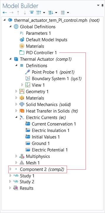
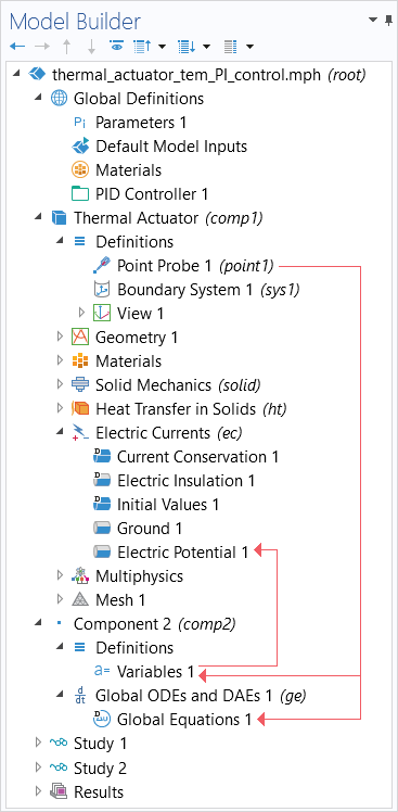
The PID Controller add-in enables us to easily set up a PI (or PID) controller for our device, and is what creates the 0D model component with the ordinary differential equations for the PI controller. It is set up for a reasonable controller response with allowed electric potentials between 0 V and 25 V (settings pictured below). The physics are coupled between the components by including the variables generated and definitions created in either model component into the settings of the other model component.

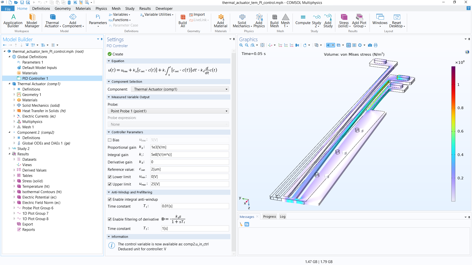A screenshot of the thermal microactuator model with PI control, with the settings for the PID Controller add-in displayed.

The process of creating this transient, multicomponent version of the thermal microactuator tutorial model is as follows:

1. Set up the model and run the study
   • Use the fully automatic approach to model the device in a 3D model component
2. Create definitions for PI control
   • Define a point probe at the tip of the actuator
3. Use the PID Controller add-in
   • Define the controller parameters
4. Implement physics couplings between model components
   • Use the manual approach with user-defined couplings to set up a feedback loop into the model
5. Run the study and check the results

Building and setting up this model using the fully automatic approach is covered in a separate Learning Center article on that topic, while using the PID Controller add-in is introduced and detailed in a blog post. As such, those details of the model build are omitted here for brevity, as we want to focus on Step 4 of the list: the coupling of the physics between the model components.

Coupling Between Components

As noted previously, we want the input (the electric potential) to change based on the computed solution for the displacement of the device. To monitor the displacement of the actuator and use it as feedback to the PI controller, we define a Point Probe at the farthermost tip in the geometry and enter the expression for the displacement magnitude as the quantity to monitor.

The COMSOL Multiphysics UI showing the Model Builder, Point Probe Settings window, and Graphics window, which is displaying the model. The settings for the Point Probe that was defined to monitor the displacement of the microactuator.

This point probe is then selected as the probe to use for the PI Controller. When creating the PID Controller, a 0D model component is generated that includes the point probe in the equations and expressions for the variables. This results in the coupling of the measured displacement, which is monitored by the probe from the 3D model of the device, with the 0D PI controller model component.

The COMSOL Multiphysics UI showing the Model Builder with Global Equations 1 highlighted and the Global Equations settings.
The ODEs for the PI controller, which includes the point probe in the expression.

The COMSOL Multiphysics UI showing the Model Builder and the Variables Settings window.
The variables for the 0D model component, which includes the point probe in the expression.

Also upon generating the model component, the control variable u_in_ctrl for the PI controller is available to use. The control variable is the electric potential input to the device and thus is entered in the expression for the Electric Potential boundary condition of the 3D model component — thereby coupling the varying electrical input controlled by the PI controller in the 0D model component with the device in the 3D model component.

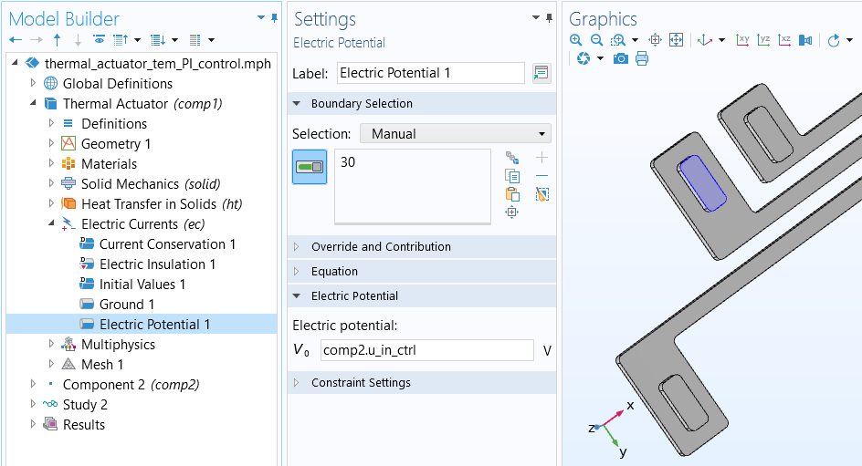
The Settings window for the Electric Potential boundary condition.

In the following tutorial video, you can see a demonstration of this implementation of the manual approach with user-defined couplings, wherein we couple the physics for a multiphysics model between multiple model components.

Tutorial: Modeling a Thermal Microactuator with PI Control

Further Learning

There are various ways in which you can couple the physics between model components. If you are interested in finding COMSOL Multiphysics^® models that contain multiple model components and are relevant to what you are modeling, we recommend searching comp2 in the Application Libraries. You can then navigate to the appropriate application area for the physics you are simulating.

If you are interested in learning more about using the PID Controller add-in, we recommend our blog post "How to Simulate Control Systems Using the PID Controller Add-In". The tutorial model discussed in the post, Process Control Using a PID Controller, demonstrates coupling the physics among multiple components.

If you are interested in learning more about the use of extrusion operators, you can see the "Nonlocal Couplings and Coupling Operators" chapter in the COMSOL Reference Manual documentation. If you are specifically interested in models that include multiple components and include the use of the General Extrusion operator, we recommend searching comp2 @tag:genext in the Application Libraries. We also recommend the following resources:

• Examples of the General Extrusion Operator
• Accessing Nonlocal Variables with Linear Extrusion Operators
• Part 2: Mapping Variables with General Extrusion Operators
• Postprocessing Local Data Using Component Coupling