学习中心

Examples of the withsol Operator

---

Thewithsoloperator allows you to extract the solution from any solver sequence in the current model and use it in other studies, or during postprocessing.

Comparing the Results Between Two Studies

Let us consider a simple thermal example. A steady-state simulation of a square with a temperature of 20ºC on the left-hand side. We run two studies in the model. One where the temperature on the right-hand side is 100ºC (Study 1) and one where the temperature is 200ºC (Study 2). To evaluate the temperature difference between the two studies, we can use thewithsoloperator.

The basic form of thewithsoloperator is:withsol('tag',expr), where'tag'is the tag of the solver sequence we want to extract the solution from, andexpris the expression we want to evaluate. To be able to see the tag, make sure thattagis selected from theModel Tree Node Textmenu at the top of theModel Builderwindow. The tag for each node appears in curly brackets {} after the node name.

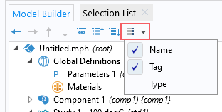
TheModel Tree Node Textmenu, with theNameandTagoptions enabled.

To see the difference between the temperatures inStudy 2andStudy 1, we create a plot for the Study 2 dataset, and use the expressionT-withsol('sol1',T).

A screenshot of the model tree, with the Solution 1 and Surface 1 nodes highlighted, and the Surface Settings window with the withsol Expression highlighted. The operator used in the expression for aSurface plot node, which defines the temperature difference between the solution from the second study and solution from the first study.

In this expression, the variable Toutside of the withsoloperator is taken from Study 2(with the tag 'sol2'), whereas the withsoloperator picks up the temperature from Study 1, which has the tag 'sol1'. The resulting plot shows the temperature difference across the domain, with the difference being 0 at the end where the temperature is the same in both studies.

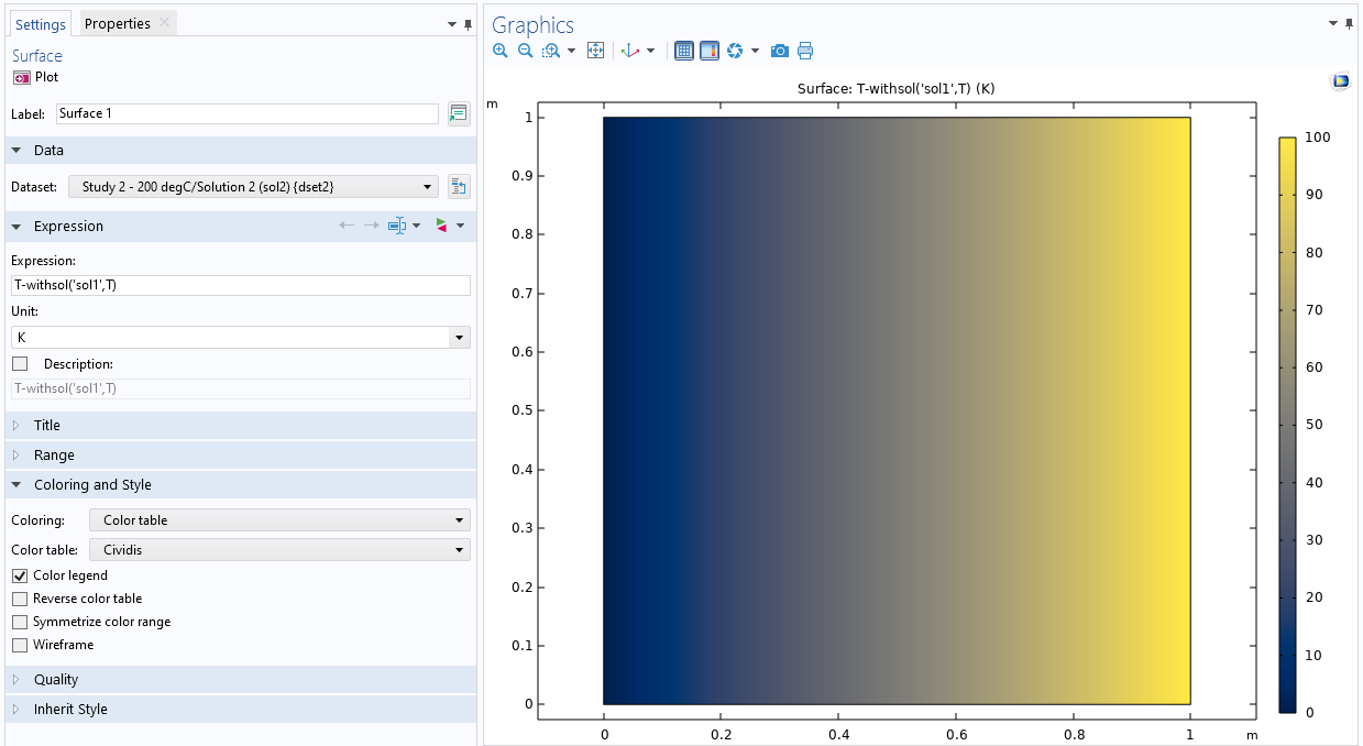A screenshot of the Surface Settings window on the left and the Graphics window with a temperature plot on the right.
The settings for one of theSurface plot nodes, wherein the operator and utilized, and the resulting plot in theGraphics window.

Comparing the Results Between Two Parameter Values in the Same Study

It is also possible to compare results between two parameters in the same study or between two times in a transient study. If we, instead of using two studies in our example, use only one study with a parameterized temperature on the right-hand side, we can similarly find the difference between the two temperatures. However, we need to use an expanded version of thewithsoloperator to not only specify which solution we want to extract results from, but also which parameter value. This time, the operator will look like this:

withsol('tag',expr, setval(par,value))

Here,'tag', andexprare the same as before. What is new issetval(par,value). The operatorsetvalis an operator commonly used together withwithsolto specify which value the parameterparshould have.

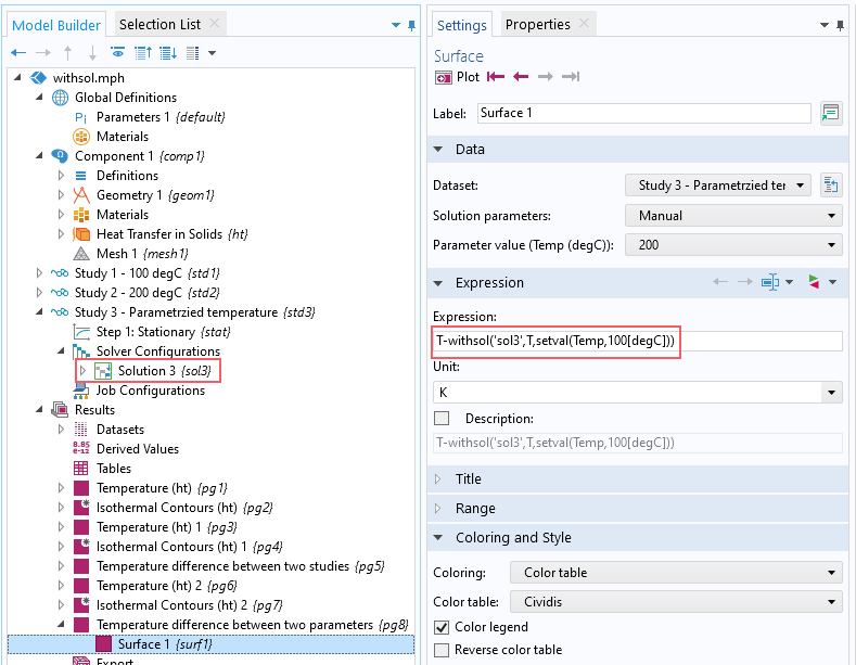A screenshot of the model tree on the left, with the Solution and Surface nodes selected, and the Surface Settings window on the right, with the Expression highlighted and including the withsol and setval operators. TheSettings window for one of theSurface plot nodes, wherein thewithsol andsetval operators are used in the expression. The solution forStudy 3 is included in the expression and is highlighted in theModel Builder window.

Here,Tis taken from the setting for our plot, soStudy 3and a parameter value of 200ºC. Thewithsoloperator picks up the values of the variableTfrom the same study (with the tag'sol3'), but when the parameterTempis 100ºC. This is done by setting the value of the parameterTempto '100[degC]' with thesetvaloperator. This plot gives the same result as the plot above.

Please note that while this can be accomplished with the expanded use of thewithsoloperator outlined above, there are other more efficient options also available. When comparing results inside the same solution, the at operator using the expressionat(,expr)and with operator using the expressionwith( ,expr) are preferred. Since they don’t need to map solutions from one solution/xmesh to another and just read from another position in the same solution, this method can be expected to be faster. Additionally, the syntax involved is simplified since you don't need to know the solution tag and don't need to use thesetvaloperator.

Using Results from One Study as Input in Another

In the modelSlope Stability in an Embankment Dam, thein situstresses from pore pressure and gravity are calculated, and the results from that study are used as an initial stress for the safety factor calculation. Thein situstresses are accessed using thewithsoloperator.

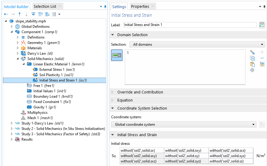A screenshot of the model tree and Settings window for the Initial Stress and Strain feature. TheSettings window for theInitial Stress and Strain feature, wherein thewithsol operator is used.

It is additionally possible to use thesetindandsetvaloperators as additional arguments to thewithsoloperator. These operators work with results from a time-dependent solver, an eigenvalue solver, a frequency sweep, or an Auxiliary sweep over one or more more parameters.

Thesetindoperator indexes into the time-domain solution, or the index of the list of eigenvalues, or the index into a sweep over frequency or any other parameter. Positive indices start from the beginning, and negative from the end of the list.

For example, when working with time-domain solutions:

withsol('sol1',expr,setind(t,1))will return the first timestep. Alternatively, usewithsol('sol1',expr,setind(t,'first'))

withsol('sol1',expr,setind(t,2))will return the second timestep.

withsol('sol1',expr,setind(t,-2))will return the second-to-last timestep.

withsol('sol1',expr,setind(t,-1))will return the last timestep. Alternatively, usewithsol('sol1',expr,setind(t,'last'))

For eigenvalue solutions, the index variable islambda, and for frequency sweep the frequency variable isfreq.

Thesetvaloperator instead extracts the solution at a user-specified value, and interpolates between stored time-domain solutions. For example:

withsol('sol1',expr,setval(t,0.5))will return the solution at time of 0.5 seconds. If there is no stored data at this timestep, then a solution is interpolated from the nearest stored timesteps. This interpolation will make usage of the time derivatives, if they are stored as shown in the screenshot below of theTime-Dependent Solver. A Hermite interpolation is used if time derivatives are available, otherwise linear interpolation is used. If a value outside of the time range is specified then the nearest timestep (first or last) is used.

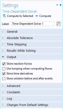
Within theTime-Dependent Solversettings, the default option is to store time derivatives.

When used in conjunction with eigenvalue solutions, the setval operator will return a solution that is within a tolerance of the actual eigenvalue. For example:
withsol('sol1',expr, setval(lambda,-100i))will return the solution even if the eigenvalue is actually -100.01i.

When used with a frequency sweep or auxiliary sweep, the exact numeric value of the frequency or parameter must be specified. If sweeping over multiple frequencies and/or parameters, it is possible to pass multiple arguments to setval, as well as setind, to make the syntax more compact. For example:
withsol('sol1',expr, setval(freq,60,param,5))is equivalent towithsol('sol1',expr, setval(freq,60),setval(param,5)).

More Advanced Usage of the withsol Operator

For an example of more advanced usage of thewithsoloperator, see the modelBracket - General Periodic Dynamic Analysis. You can find it among the tutorials for the Structural Mechanics Module in the Application Library in the following files:

• bracket_general_periodic.mph
• models.sme.bracket_general_periodic.pdf

In that model, thewithsoloperator is used to extract frequency-dependent loads from one study and use them as input for the corresponding frequencies in a second study.