Defining Multiphysics Models Manually with Predefined Couplings
When defining the physics for a multiphysics model, you may want to use an incremental strategy where you include one single physics interface at a time and then manually add all the predefined multiphysics couplings. In COMSOL Multiphysics®, we call this simulation strategy the manual approach using predefined couplings. This contrasts from thefully automatic approach, which involves an automated implementation, and is comparable to themanual approach with user-defined couplings, which involves a more manual implementation. In this article, we will explain the manual approach with predefined couplings and detail its use further.
When to Use the Manual Approach with Predefined Couplings
Each physics phenomena described in a multiphysics model may contain complex operating conditions, material properties, initial conditions, and boundary conditions. These have to be defined in the physics settings for each physics interface included in the model.
In order to control each step of the modeling process, it may be good to introduce one physics phenomenon at a time and check the results for every added phenomenon. This sequential bootstrapping strategy gives you a better chance to catch any errors in your formulation of the problem and in entering the settings in the COMSOL Multiphysics®user interface (UI). In addition, solving the full multiphysics model equations every time you want to check if a formulation or input for one of the physics interfaces is correct may be very time consuming and computationally expensive. Using this approach enables you to examine and validate both the implementation of and results for each physics.
The manual approach using predefined couplings is this such strategy. A single physics interface is added at a time and the predefined multiphysics couplings are added manually as more coupled physics interfaces are added. Hence, you are building up to the full multiphysics model. This sequential strategy becomes increasingly more useful as the models you're working on increase in complexity and involve more physics interfaces. The logic used for employing the approach, as well as the steps to implement it, are explained below.
Procedure to Implement the Approach
The sequence of steps in the manual approach involves adding, setting up, and computing the solution to the constituent physics interfaces or combinations of physics interfaces in your model. The process is then repeated until you have completed the setup for all physics interfaces and multiphysics couplings.
The purpose of the sequential modeling strategy is to compartmentalize the model-building process to make it easier. As such, a general outline of the procedure for using the sequential approach is as follows:
- Add the physics interface
- Define the physics settings
- Define the multiphysics couplings (only available when multiple physics interfaces have been added)
- Open theAdd Multiphysicswindow
- Add the appropriate multiphysics couplings to combine participating physics interfaces
- Add a separate study for the multiphysics model
- Compute the study
- Check the results
- Repeat steps 1–4 for each subsequent combination of physics
Multiphysics couplings are available to be added once your model component contains more than one physics interface. At this time, aMultiphysicsnode automatically appears in the model tree. Through either this node or the respective button in thePhysicsribbon tab, you are able to prompt theAdd Multiphysicswindow to appear. When opened, you are able to select or deselect which physics interfaces you want to couple. Based on the combination of physics interfaces you choose to couple, different multiphysics couplings will be available (as pictured below). At minimum, at least two physics interfaces need to be selected in order for a multiphysics coupling option to appear in theAdd Multiphysicswindow.
 3 side-by-side screenshots showing the Add Multiphysics window and different multiphysics couplings you can implement in a model.
Using theAdd Multiphysics window to implement multiphysics couplings between the respective physics interfaces. Note that different couplings are available based on the combination of physics interfaces selected.
In another article discussing thefully automatic approachfor defining multiphysics models, a noteworthy benefit discussed is that the optimal study and solver settings for the combination of physics interfaces in your model are automatically handled. TheAdd Multiphysicswindow gives you the same benefit as when you add physics interfaces manually one-by-one. When a multiphysics coupling is added to your model component through these means, the software automatically adjusts the settings for each participating physics interface. This enables you to still take advantage of the functionality even if you are not using the fully automatic approach.
Below, we demonstrate use of the approach with a tutorial model serving as our multiphysics example.
Walkthrough Example: Modeling Resistive Heating and Thermal Expansion
To demonstrate using the approach, we can revisit the thermal-electrical-mechanical ("tem") version of thethermal microactuator tutorial model, which is found in the Application Library under theMultiphysicssection of theCOMSOL Multiphysicsfolder. It is assumed that all details regarding the model setup, except for the physics settings, have been completed, and we will specifically focus on defining the multiphysics couplings in the model.
Since we are employing a sequential strategy, we first need to determine the order of the separate analyses. In a microactuator, an electric potential is applied over the anchors of the two hot arms. As current flows through the hot arms, resistive heating heats them up, causing thermal expansion. The cold arm does not expand to the same extent and this results in the deformation, in the negativeydirection, of the actuator.
This means that the process starts with the electric potential, continues with the induced current causing a temperature increase, which in turn causes the structural deformation. The natural order of the physics phenomena occurring dictate the order of the analyses:
- Performing an electrical analysis
- Conducting an electrical-thermal analysis
- Solving the equations for the full multiphysics model, which accounts for electrical, thermal, and structural effects
It should be noted, however, that in general, when using this approach, we can add and define the physics interfaces in any order. In this case, only one specific order makes sense, since computing the thermal model without a current would just give a uniform temperature field. Without a varying temperature field, the actuator does not move and it is meaningless to perform the structural analysis. Let's now dive into implementing the sequential approach with the plan above.
The Electrical Analysis
For the electrical analysis, we start by adding theElectric Currentsinterface to the model component and define the physics settings by adding the boundary conditions. Then, using the stationary study previously added, we compute and obtain the results for the electric potential of the microactuator.
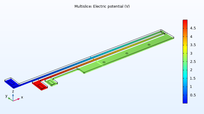
Electric potential results plot for the electrical analysis of the microactuator.
After computing the study for this first single-physics model, we want to verify that the results are accurate. If they are, we can proceed with performing our second study, the electrical-thermal analysis. If they are not, we would then take this time to trace and correct any faults in our model. As seen above, the results show an electric potential range of 0–5 volts throughout the device, with the highest observed at the middle hot arm's anchor and the lowest at the long hot arm's anchor. These results are consistent with how we defined the physics and are what we would expect, since an electric potential of 5 volts was applied to the middle hot arm's anchor and was ground at the long hot arm's anchor, while all other surfaces were electrically insulated.
The Electrical-Thermal Analysis
Having confirmed our results for the electrical analysis of the microactuator, we can move forward and repeat this process for the electrical-thermal analysis of the device. To keep the results organized, it would be best to use multiple studies. We add a new stationary study to the model component, using the study to solve for both the electric and heat transfer interface equations. To do this, we add theHeat Transfer in Solidsinterface to the model component. Once again, we add the physics nodes needed to define the heat transfer in the microactuator. Thereafter, we need to implement a multiphysics coupling to couple the physics interfaces. To do this, we can open theAdd Multiphysicswindow, choose both physics interfaces to be coupled, choose only the second study under theSolvecolumn, select theJoule Heating, and then add it to the component.
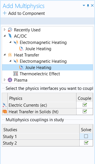
TheAdd Multiphysicswindow with the selections for the electrical-thermal analysis, as specified above.
Now, we can compute the second study in our model component. Upon solving, we are provided with both temperature and isothermal contour plots showing the temperature distribution in the microactuator.
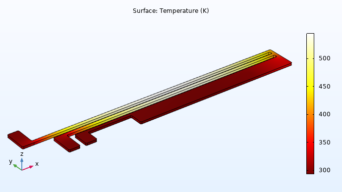
Temperature plot for the electrical-thermal analysis of the microactuator.
Once again, we examine the results. If they are accurate and the model is behaving as we expect it to be, we can proceed. Here, the maximum temperature is observed between the two hot arms. As we move toward the anchors of the hot arms or the cold arm, there is minimal — if any — temperature rise. These results are appropriate, as the electric potential was applied between the two hot arms, wherein heat is generated through resistive losses. The actuator also experiences convective cooling over all boundaries through a thin air layer, which reduces the temperature closer to ambient temperature.
The Electrical-Thermal-Structural Analysis
At this point, we progress to the full multiphysics model, which includes the structural effects. Let's begin by adding theSolid Mechanicsinterface as our third physics interface in the model component. Next, we need to add a new stationary study in which all three physics interfaces are selected to be solved for. Following this, we implement the multiphysics effect necessary to couple heat transfer and solid mechanics. We do this by opening theAdd Multiphysicswindow, selecting those two respective physics interfaces to couple, and selecting theThermal Stress, Solidmultiphysics coupling. To keep our structural, thermal, and multiphysics analyses separate, we only have the couplings solved for in the third study.
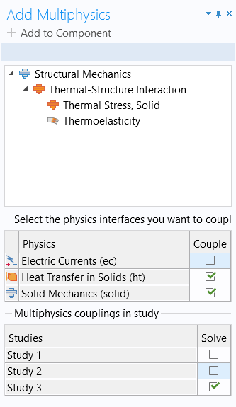
TheAdd Multiphysicswindow with the selections for the full multiphysics analysis, as specified above.
Now, we can select theStudy 3node, computing it to solve the model equations. When it has finished solving, three new results plots are generated that display the electrical, thermal, and structural results of the microactuator. Selecting the newly generated stress plot reveals that thermally induced stresses and strains develop between the two hot arms, causing them to expand and bend the actuator.
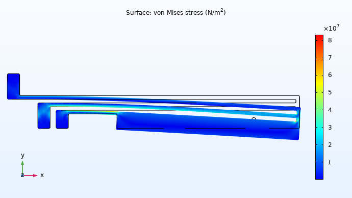
Von Mises stress distribution results for the multiphysics analysis of the thermal microactuator. The black geometry outline shows the original configuration of the actuator geometry, indicating the degree to which it deforms due to thermal expansion. Note that a deformation scale factor of approximately 6.6 is used.
To see the step-by-step process in detail for using this approach, you can watch the video below for a full demonstration.
Tutorial: Defining a Multiphysics Model Using the Manual Approach with Predefined Couplings
Modeling Exercises
Demonstrate the knowledge you have gained from this article by putting it into practice with the follow-up modeling exercises listed below. The directions provided for each modeling exercise contain all the information necessary in order to complete it, but are intentionally generalized to encourage self-guided problem-solving. You can check your implementation with the solution model files provided by comparing them manually or using theComparison toolto exactly identify the differences.
- In Part 1 of this course, you built the busbar tutorial model using the fully automatic approach. Now, use the manual with predefined couplings approach to define the physics for this model. Use the followingdocumentfor reference to define the physics setup. The geometry is available to download:busbar.mphbin.
- In Part 1 of this course, you built the free convection tutorial model using the fully automatic approach. Now, use the manual with predefined couplings approach to define the physics for this model. Use the followingdocumentfor reference to define the physics setup. The geometry is available to download:free_convection.mphbin.
- Follow thedirectionsprovided to build the convective cooling of a busbar tutorial model using the manual approach with predefined couplings. The geometry file is available to download:busbar_box.mphbin.
请提交与此页面相关的反馈,或点击此处联系技术支持。
